6. Basis sets for fitting#
As outlined in Part I, particularly Chpt. 3, in order to compute and/or retrieve a set of matrix elements from experimental results, various physical properties of the system at hand are required. In particular, the symmetry of the system, the ionizing channel(s) of interest, and the properties of the ionizing radiation are all required to define the basis set used for radial matrix elements retrieval via fitting (Chpt. 4).
Numerically, there are two main methods to do this demonstrated herein:
The use of symmetry to define the basis set, in terms of symmetry-allowed components.
The use of ab initio calculations to define the basis functions. In the work presented here, it is specifically ePolyScat (ePS) [36, 37, 38, 39] matrix elements that are used, since these are also used to generate the synthetic data used to test the bootstrap retrieval protocol.
Manual creation of basis sets is also possible, and may be useful in some cases, particularly when exploring limiting cases.
6.1. Symmetry-defined basis sets#
As illustrated in Sect. 3.2, a set of symmetry-allowed continuum functions can be determined, corresponding to a given ionizing transition and specific dipole symmetries. Such a basis set defines the allowed matrix elements in terms of a set of symmetrized harmonics, and these can be used as a basis for fitting with only minimal knowledge of the system required.
The main advantage of a purely symmetry-defined approach is that no additional ab initio computations are required, and that the resulting basis set is general. As discussed and illustrated in Sect. 3.3, the resulting channel functions can also be used to guide analysis (and experiment if available prior to experimental work). The main disadvantage of such a blind approach is that initial data analysis may require significantly more effort than working from a computationally-defined basis, in particular the initial fitting space may be larger than required (leading to computationally more-demanding fitting runs), and testing for contributing/non-negligible terms by, e.g. using varying \(l_{max}\), may be required in initial fitting runs. For further discussion, see Quantum Metrology Vols. 1 & 2 [4, 9].
6.2. Computationally-defined basis sets#
In cases where photoionization calculations are available, the results can also be used to determine allowed basis components. Use of ab initio computational results is, of course, useful for simulation as well as direct analysis, and may lead to a reduced basis set relative to the symmetry-defined case, since some components may be small and can be ignored. However, it does also require that substantial calculations are performed (or results are available, e.g. from ePSdata [48]), and - potentially - may bias the matrix element analysis/retrieval in cases where the experimental results and computational results are significantly different.
6.3. Basis creation worked examples#
In the case study chapters, basis functions are created for each case at hand, typically starting from ab initio computational results (since these are required to simulate the sample data). Here a more detailed worked example is given to illustrate the basic methodology behind the assignments, the differences between the approaches, and highlight some issues of convention which may arise.
6.3.1. Simple case: \(N_2~3\sigma_g^{-1}\) ionization#
As a simple example, consider the case of a homonuclear diatomic (\(D_{\infty h}\) PG, cylindrically symmetric), and a totally symmetric ionizing orbital, e.g. the ionization of the \(\Sigma_{g}^{+}\) HOMO of \(N_2\). For this example,
\(\Gamma^{i} = \Gamma^{+} = \Gamma^{s} = \Sigma_{g}^{+}\). Note that, for single-electron ionization from a fully-occupied valence orbitals, the ion symmetry will correspond to the hole symmetry, hence the symmetry of the ionized orbital. This simple picture may break down for more complicated cases, e.g. if multi-electron effects or substantial nuclear motions are involved; for radical systems the overall symmetry of all partially-occupied orbitals must be accounted for.
The dipole symmetries correspond to the Cartesian axes/translations given in the character tables, hence \(\Sigma_{u}^{+} = (z)\) and \(\Pi_{u} = (x,y)\) for \(D_{\infty h}\). Note that, in this cylindrically symmetric case, the Cartesian \((x,y)\) components are spanned by the doubly-degenerate \(\Pi_{u}\) irreducible representation - physically this corresponds to the arbitrary orientation of these axes in the MF (i.e. no preferred direction is defined).
Following Eq. (3.12), the allowed components (irreducible representations) can be determined by hand making use of character and direct product tables, and substituting in for the terms defined above:
Hence the allowed continuum components are given by:
As indicated above, this case is split by symmetry into a “parallel” and “perpendicular” continua, accessed by the \(z\) or \((x,y)\) dipole components in the MF respectively; these are often denote generically by appending \(\perp\) and \(\parallel\) symbols to derived quantities, e.g. \(\sigma_{\parallel}\) for the corresponding cross-section. In the LF or AF these continua can be mixed according to the polarization state and geometry of the ionizing radiation, and the molecular alignment (ADMs).
The total scattering state symmetry is often also used to label continuum states, and is given by \(\Gamma_{\mathrm{scat}}=\Gamma^{+}\otimes\Gamma^{e}\):
This is identical to \(\Gamma^{e}\) in this simple case.
6.3.2. Degenerate case example: \(N_2~3\pi_u^{-1}\) ionization#
For more complicated cases, multiple symmetry components may be found. For example, the ionization from a \(\Pi_u\) orbital, e.g. \(N_2\) HOMO-1.
In this case, \(\Gamma^{+} = \Pi_u\), and - working through the direct products as above - yields the allowed continuum components:
And total scattering state symmetries:
In this case, the direct product results give multiple components for each continua. However, since the continuum wavefunction is already defined for multiple components, as given by \(\Gamma^{e}\), only the first \(\Gamma_{\mathrm{scat}}\) symmetry is required as a unique label here. In this case, therefore, \(\Gamma_{\mathrm{scat}} = \Pi_{u}~(x,y)\) and \(\Gamma_{\mathrm{scat}} =\Sigma_{u}^{+}~(z)\) suffice to label the total scattering states.
6.3.3. Defining symmetrized harmonics#
In the examples above, the allowed irreducible representations are defined by hand from direct product tables for illustrative purposes. But, in general, it is tedious to categorize/define the allowed spherical harmonics and linear combinations. With the Photoelectron Metrology Toolkit [5], both the direct products illustrated above, and the determination of associated spherical harmonics, can be automated and the full basis set rapidly defined numerically. This was illustrated briefly in Sect. 3.2, and is extended here for the example cases above.
Computationally, the cylindrically-symmetric \(\infty\) groups can be approximated by a high-order group, e.g. \(D_{\infty h} \approx D_{10h}\). (For a cross-check, see the full tables and direct products online.) Here the notational convention is \(A1 = \Sigma^{+}\), \(A2 = \Sigma^{-}\), \(E1 = \Pi\), \(E2 = \Delta\) and so forth (see the \(D_{\infty h}\) character table for more details).
Show code cell content
# Run default config - may need to set full path here
%run '../scripts/setup_notebook.py'

# Override plotters backend?
# plotBackend = 'pl'
*** Setting up notebook with standard Quantum Metrology Vol. 3 imports...
For more details see https://pemtk.readthedocs.io/en/latest/fitting/PEMtk_fitting_basic_demo_030621-full.html
To use local source code, pass the parent path to this script at run time, e.g. "setup_fit_demo ~/github"

*** Running: 2023-12-07 10:50:36
Working dir: /home/jovyan/jake-home/buildTmp/_latest_build/html/doc-source/part2
Build env: html
None

* Loading packages...
* sparse not found, sparse matrix forms not available.
* natsort not found, some sorting functions not available.
* Setting plotter defaults with epsproc.basicPlotters.setPlotters(). Run directly to modify, or change options in local env.
* Set Holoviews with bokeh.
* pyevtk not found, VTK export not available.
* Set Holoviews with bokeh.
Jupyter Book      : 0.15.1
External ToC      : 0.3.1
MyST-Parser       : 0.18.1
MyST-NB           : 0.17.2
Sphinx Book Theme : 1.0.1
Jupyter-Cache     : 0.6.1
NbClient          : 0.7.4
# Example following symmetrized harmonics demo

# Import class
from pemtk.sym.symHarm import symHarm

# Compute hamronics for D10h, lmax=4
sym = 'D10h'
lmax=4

symObjA1g = symHarm(sym,lmax)

# Allowed terms and mappings are given in 'dipoleSyms'
# symObj.dipole['dipoleSyms']
*** Mapping coeffs to ePSproc dataType = matE
Remapped dims: {'C': 'Cont', 'mu': 'it'}
Added dim Eke
Added dim Targ
Added dim Total
Added dim mu
Added dim Type
Found dipole symmetries:
{'A2u': {'m': [0], 'pol': ['z']}, 'E1u': {'m': [-1, 1, -1, 1], 'pol': ['x', 'y']}}
# Setting the symmetry for the neutral and ion allows direct products to be computed,
# and allowed terms to be determined.

sNeutral = 'A1g'
sIonSG = 'A1g'

symObjA1g.directProductContinuum([sNeutral, sIonSG])

# Results are pushed to self.continuum, in dictionary and Pandas DataFrame formats,
# and can be manipulated using standard functionality.
# The subset of allowed values are also set to a separate DataFrame and list.

# Glue figure for later - real part only in this case
# Also clean up axis labels from default state labels ('LM' and 'LM_p' in this case).
glue("dipoleTermsD10hA1g", symObjA1g.continuum['allowed']['PD'])
Show code cell output
| allowed | m | pol | result | terms | ||
|---|---|---|---|---|---|---|
| Dipole | Target | |||||
| A2u | A1g | False | [0] | ['z'] | ['A2u'] | ['A1g', 'A1g'] |
| A2g | False | [0] | ['z'] | ['A1u'] | ['A1g', 'A1g'] | |
| A1u | False | [0] | ['z'] | ['A2g'] | ['A1g', 'A1g'] | |
| A2u | True | [0] | ['z'] | ['A1g'] | ['A1g', 'A1g'] | |
| B1g | False | [0] | ['z'] | ['B2u'] | ['A1g', 'A1g'] | |
| B1u | False | [0] | ['z'] | ['B2g'] | ['A1g', 'A1g'] | |
| B2g | False | [0] | ['z'] | ['B1u'] | ['A1g', 'A1g'] | |
| B2u | False | [0] | ['z'] | ['B1g'] | ['A1g', 'A1g'] | |
| E1u | False | [0] | ['z'] | ['E1g'] | ['A1g', 'A1g'] | |
| E1g | False | [0] | ['z'] | ['E1u'] | ['A1g', 'A1g'] | |
| E2g | False | [0] | ['z'] | ['E2u'] | ['A1g', 'A1g'] | |
| E2u | False | [0] | ['z'] | ['E2g'] | ['A1g', 'A1g'] | |
| E3u | False | [0] | ['z'] | ['E3g'] | ['A1g', 'A1g'] | |
| E3g | False | [0] | ['z'] | ['E3u'] | ['A1g', 'A1g'] | |
| E4g | False | [0] | ['z'] | ['E4u'] | ['A1g', 'A1g'] | |
| E4u | False | [0] | ['z'] | ['E4g'] | ['A1g', 'A1g'] | |
| E1u | A1g | False | [-1, 1, -1, 1] | ['x', 'y'] | ['E1u'] | ['A1g', 'A1g'] |
| A2g | False | [-1, 1, -1, 1] | ['x', 'y'] | ['E1u'] | ['A1g', 'A1g'] | |
| A1u | False | [-1, 1, -1, 1] | ['x', 'y'] | ['E1g'] | ['A1g', 'A1g'] | |
| A2u | False | [-1, 1, -1, 1] | ['x', 'y'] | ['E1g'] | ['A1g', 'A1g'] | |
| B1g | False | [-1, 1, -1, 1] | ['x', 'y'] | ['E4u'] | ['A1g', 'A1g'] | |
| B1u | False | [-1, 1, -1, 1] | ['x', 'y'] | ['E4g'] | ['A1g', 'A1g'] | |
| B2g | False | [-1, 1, -1, 1] | ['x', 'y'] | ['E4u'] | ['A1g', 'A1g'] | |
| B2u | False | [-1, 1, -1, 1] | ['x', 'y'] | ['E4g'] | ['A1g', 'A1g'] | |
| E1u | True | [-1, 1, -1, 1] | ['x', 'y'] | ['A1g', 'A2g', 'E2g'] | ['A1g', 'A1g'] | |
| E1g | False | [-1, 1, -1, 1] | ['x', 'y'] | ['A1u', 'A2u', 'E2u'] | ['A1g', 'A1g'] | |
| E2g | False | [-1, 1, -1, 1] | ['x', 'y'] | ['E1u', 'E3u'] | ['A1g', 'A1g'] | |
| E2u | False | [-1, 1, -1, 1] | ['x', 'y'] | ['E1g', 'E3g'] | ['A1g', 'A1g'] | |
| E3u | False | [-1, 1, -1, 1] | ['x', 'y'] | ['E2g', 'E4g'] | ['A1g', 'A1g'] | |
| E3g | False | [-1, 1, -1, 1] | ['x', 'y'] | ['E2u', 'E4u'] | ['A1g', 'A1g'] | |
| E4g | False | [-1, 1, -1, 1] | ['x', 'y'] | ['B1u', 'B2u', 'E3u'] | ['A1g', 'A1g'] | |
| E4u | False | [-1, 1, -1, 1] | ['x', 'y'] | ['B1g', 'B2g', 'E3g'] | ['A1g', 'A1g'] |
| allowed | m | pol | result | terms | ||
|---|---|---|---|---|---|---|
| Dipole | Target | |||||
| A2u | A2u | True | [0] | [z] | [A1g] | [A1g, A1g] |
| E1u | E1u | True | [-1, 1, -1, 1] | [x, y] | [A1g, A2g, E2g] | [A1g, A1g] |
Fig. 6.1 Dipole-allowed continuum symmetries (“Target”) for \(D_{10h}\), \(A_{1g}\) ionization.#
# Setting the symmetry for the neutral and ion allows direct products to be computed,
# and allowed terms to be determined.

sNeutral = 'A1g'
sIonPU = 'E1u'

# Define new object for E1u case
symObjE1u = symHarm(sym,lmax)
symObjE1u.directProductContinuum([sNeutral, sIonPU])

# Results are pushed to self.continuum, in dictionary and Pandas DataFrame formats,
# and can be manipulated using standard functionality.
# The subset of allowed values are also set to a separate DataFrame and list.

# Glue table for later
glue("dipoleTermsD10hE1u", symObjE1u.continuum['allowed']['PD'])
Show code cell output
*** Mapping coeffs to ePSproc dataType = matE
Remapped dims: {'C': 'Cont', 'mu': 'it'}
Added dim Eke
Added dim Targ
Added dim Total
Added dim mu
Added dim Type
Found dipole symmetries:
{'A2u': {'m': [0], 'pol': ['z']}, 'E1u': {'m': [-1, 1, -1, 1], 'pol': ['x', 'y']}}
| allowed | m | pol | result | terms | ||
|---|---|---|---|---|---|---|
| Dipole | Target | |||||
| A2u | A1g | False | [0] | ['z'] | ['E1g'] | ['A1g', 'E1u'] |
| A2g | False | [0] | ['z'] | ['E1g'] | ['A1g', 'E1u'] | |
| A1u | False | [0] | ['z'] | ['E1u'] | ['A1g', 'E1u'] | |
| A2u | False | [0] | ['z'] | ['E1u'] | ['A1g', 'E1u'] | |
| B1g | False | [0] | ['z'] | ['E4g'] | ['A1g', 'E1u'] | |
| B1u | False | [0] | ['z'] | ['E4u'] | ['A1g', 'E1u'] | |
| B2g | False | [0] | ['z'] | ['E4g'] | ['A1g', 'E1u'] | |
| B2u | False | [0] | ['z'] | ['E4u'] | ['A1g', 'E1u'] | |
| E1u | False | [0] | ['z'] | ['A1u', 'A2u', 'E2u'] | ['A1g', 'E1u'] | |
| E1g | True | [0] | ['z'] | ['A1g', 'A2g', 'E2g'] | ['A1g', 'E1u'] | |
| E2g | False | [0] | ['z'] | ['E1g', 'E3g'] | ['A1g', 'E1u'] | |
| E2u | False | [0] | ['z'] | ['E1u', 'E3u'] | ['A1g', 'E1u'] | |
| E3u | False | [0] | ['z'] | ['E2u', 'E4u'] | ['A1g', 'E1u'] | |
| E3g | False | [0] | ['z'] | ['E2g', 'E4g'] | ['A1g', 'E1u'] | |
| E4g | False | [0] | ['z'] | ['B1g', 'B2g', 'E3g'] | ['A1g', 'E1u'] | |
| E4u | False | [0] | ['z'] | ['B1u', 'B2u', 'E3u'] | ['A1g', 'E1u'] | |
| E1u | A1g | True | [-1, 1, -1, 1] | ['x', 'y'] | ['A1g', 'A2g', 'E2g'] | ['A1g', 'E1u'] |
| A2g | True | [-1, 1, -1, 1] | ['x', 'y'] | ['A1g', 'A2g', 'E2g'] | ['A1g', 'E1u'] | |
| A1u | False | [-1, 1, -1, 1] | ['x', 'y'] | ['A1u', 'A2u', 'E2u'] | ['A1g', 'E1u'] | |
| A2u | False | [-1, 1, -1, 1] | ['x', 'y'] | ['A1u', 'A2u', 'E2u'] | ['A1g', 'E1u'] | |
| B1g | False | [-1, 1, -1, 1] | ['x', 'y'] | ['B1g', 'B2g', 'E3g'] | ['A1g', 'E1u'] | |
| B1u | False | [-1, 1, -1, 1] | ['x', 'y'] | ['B1u', 'B2u', 'E3u'] | ['A1g', 'E1u'] | |
| B2g | False | [-1, 1, -1, 1] | ['x', 'y'] | ['B1g', 'B2g', 'E3g'] | ['A1g', 'E1u'] | |
| B2u | False | [-1, 1, -1, 1] | ['x', 'y'] | ['B1u', 'B2u', 'E3u'] | ['A1g', 'E1u'] | |
| E1u | False | [-1, 1, -1, 1] | ['x', 'y'] | ['E1u', 'E3u'] | ['A1g', 'E1u'] | |
| E1g | False | [-1, 1, -1, 1] | ['x', 'y'] | ['E1g', 'E3g'] | ['A1g', 'E1u'] | |
| E2g | True | [-1, 1, -1, 1] | ['x', 'y'] | ['A1g', 'A2g', 'E2g', 'E4g'] | ['A1g', 'E1u'] | |
| E2u | False | [-1, 1, -1, 1] | ['x', 'y'] | ['A1u', 'A2u', 'E2u', 'E4u'] | ['A1g', 'E1u'] | |
| E3u | False | [-1, 1, -1, 1] | ['x', 'y'] | ['B1u', 'B2u', 'E1u', 'E3u'] | ['A1g', 'E1u'] | |
| E3g | False | [-1, 1, -1, 1] | ['x', 'y'] | ['B1g', 'B2g', 'E1g', 'E3g'] | ['A1g', 'E1u'] | |
| E4g | False | [-1, 1, -1, 1] | ['x', 'y'] | ['E2g', 'E4g'] | ['A1g', 'E1u'] | |
| E4u | False | [-1, 1, -1, 1] | ['x', 'y'] | ['E2u', 'E4u'] | ['A1g', 'E1u'] |
| allowed | m | pol | result | terms | ||
|---|---|---|---|---|---|---|
| Dipole | Target | |||||
| A2u | E1g | True | [0] | [z] | [A1g, A2g, E2g] | [A1g, E1u] |
| E1u | A1g | True | [-1, 1, -1, 1] | [x, y] | [A1g, A2g, E2g] | [A1g, E1u] |
| A2g | True | [-1, 1, -1, 1] | [x, y] | [A1g, A2g, E2g] | [A1g, E1u] | |
| E2g | True | [-1, 1, -1, 1] | [x, y] | [A1g, A2g, E2g, E4g] | [A1g, E1u] |
Fig. 6.2 Dipole-allowed continuum symmetries (“Target”) for \(D_{10h}\), \(E_{1u}\) ionization.#
The allowed terms can be further expressed in terms of the spherical harmonic components.
# Basis table with the Character values limited to those defined in
# self.continuum['allowed']['PD'] Target column
symObjE1u.displayXlm(symFilter = True, YlmType='comp')

# Glue table for later
glue("dipoleTermsD10hBasis", symObjE1u.displayXlm(symFilter = True,
                                                  YlmType='comp', returnPD=True))
Show code cell output
| b | ||||||||
|---|---|---|---|---|---|---|---|---|
| l | 0 | 1 | 2 | 3 | 4 | |||
| Character ($\Gamma$) | SALC (h) | PFIX ($\mu$) | m | |||||
| A1g | 0 | 0 | 0 | (1+0j) | ||||
| 1 | 0 | 0 | (1+0j) | |||||
| 2 | 0 | 0 | (1+0j) | |||||
| E1g | 0 | 0 | -1 | (0.7071067811865475+0j) | ||||
| 1 | (0.7071067811865475-0j) | |||||||
| 1 | -1 | (-0.7071067811865475-0j) | ||||||
| 1 | (0.7071067811865475-0j) | |||||||
| 1 | 0 | -1 | (0.7071067811865475+0j) | |||||
| 1 | (0.7071067811865475-0j) | |||||||
| 1 | -1 | (-0.7071067811865475-0j) | ||||||
| 1 | (0.7071067811865475-0j) | |||||||
| E2g | 0 | 0 | -2 | (0.7071067811865475+0j) | ||||
| 2 | (0.7071067811865475+0j) | |||||||
| 1 | -2 | (-0.7071067811865475+0j) | ||||||
| 2 | (0.7071067811865475+0j) | |||||||
| 1 | 0 | -2 | (0.7071067811865475+0j) | |||||
| 2 | (0.7071067811865475+0j) | |||||||
| 1 | -2 | (-0.7071067811865475+0j) | ||||||
| 2 | (0.7071067811865475+0j) | |||||||
Fig. 6.3 Dipole-allowed basis set for \(D_{10h}\), \(E_{1u}\) ionization.#
6.3.4. Mapping symmetrized harmonics to fit parameters#
The final preparatory steps for tackling a specific retrieval problem is to map the allowed channels to photoionization matrix elements - including the assignment of any missing terms - and from these to fitting paramters. The matrix elements are currently defined in the Photoelectron Metrology Toolkit [5] and the ePSproc codebase [33, 34, 35] following the definitions in ePolyScat (ePS) [36, 37, 38, 39], and the symmetry-defined cases can be remapped to this format. (Further information can be found in the PEMtk documentation [20].) For a comparison with ab initio matrix elements, see Sect. 6.4.
For symmetry-defined basis sets, these must first be mapped to an ePSproc data structure, although this step is not necessary when working from ab initio basis sets. This is explored in Sect. 6.3.4.1.
From a given basis set, the parameters used for fitting data are determined. This converts the parameters to
lmfitlibrary [66, 67] objects in magnitude-phase form, and (optionally) sets various symmetry relations and constraints. This is explored in Sect. 6.3.4.2.
Further examples can be found in the remainder of this text, and also in the PEMtk documentation [20].
6.3.4.1. Remapping to ePolyScat definitions#
In the remapping, the code attempts to assign all the symmetries matching ePolyScat definitions from the direct products. A worked example is given in the code blocks in this section, including a full output table and graphical illustration (Fig. 6.4).
The terms are:
Contis the continuum (free electron) symmetry, \(\Gamma^{e}\).Targis the target state symmetry, \(\Gamma^{+}\).Totalis the overall symmetry of the scattering state, \(\Gamma_{\mathrm{scat}}=\Gamma^{+}\otimes\Gamma^{e}\).
Additionally, the current default remapping changes some of the terms defined by the symmetrized harmonics routines and conventions:
Symmetry
C>Cont(continuum symmetry label in ePSproc)Index
h>it(degeneracy index in ePSproc)Index
mu>muX(to avoid confusion with photon indexmuin ePSproc)
Note, in particular, that \(\mu\) is - unfortunately - the photon polarization term in the conventional photoionization equations, but also used in the standard definition of the symmetrized harmonics as a degeneracy index. In some cases, the symmetrization indicies \(\mu\) or \(h\) may be redundant, and can be dropped or summed over, but care must be taken here to avoid breaking the symmetry of the simplified basis set.
Finally, the remapping adds additional labels used by ePolyScat (ePS) [36, 37, 38, 39], but which are not necessarily required in general:
Type: for ePolyScat results, this labels length or velocity gauge results; this is assigned asU(unassigned) in the conversion.Eke: the photoelectron kinetic energy, for the basis states this is just set to 0.mu: this is set to NaN by the main routine; if the ionizing channel symmetries are defined these values (the photon polarization) can be determined from the dipole-allowed terms, and this is done by theassignSymMuTerms()method, as illustrated below.
# Run conversion with a different dimMap & dataType - note this includes all symmetries,
# and both real and complex harmonic basis sets
dataType = 'matE'

# With custom dim mapping (optional)...
dimMap = {'C':'Cont', 'mu':'it'}   # Default dimMap = {'C':'Cont','h':'it', 'mu':'muX'}
# dimMap = {'C':'Cont','h':'it', 'mu':'muX'}  # Default case

# Map to ePSproc definitions
symObjA1g.toePSproc(dataType=dataType, dimMap=dimMap)

# To assign specific terms, use self.assignMissingSym
# Note this can take a single value, or a list which must match the size of the
# Sym multiindex defined in the Xarray dataset.
symObjA1g.assignMissingSym('Targ', sIonSG)

# To define terms from produts, use self.assignMissingSymProd
symObjA1g.assignMissingSymProd()

# To attempt to assign mu values (by symmetry), use self.assignSymMuTerms()
symObjA1g.assignSymMuTerms()

# Show Pandas table of results
symObjA1g.coeffs['symAllowed']['PD'].fillna('')
*** Mapping coeffs to ePSproc dataType = matE
Remapped dims: {'C': 'Cont', 'mu': 'it'}
Added dim Eke
Added dim Targ
Added dim Total
Added dim mu
Added dim Type
*** Updated self.coeffs['matE'] with new coords.
Assigned 'Total' from A1g x A1g = ['A1g']
Assigned 'Total' from A2u x A1g = ['A2u']
Assigned 'Total' from E1g x A1g = ['E1g']
Assigned 'Total' from E1u x A1g = ['E1u']
Assigned 'Total' from E2g x A1g = ['E2g']
Assigned 'Total' from E2u x A1g = ['E2u']
Assigned 'Total' from E3g x A1g = ['E3g']
Assigned 'Total' from E3u x A1g = ['E3u']
Assigned 'Total' from E4g x A1g = ['E4g']
*** Updated self.coeffs['matE'] with new coords.
Assigned dipole-allowed terms for dim = 'Cont' to self.coeffs['symAllowed']
| Cont | A2u | E1u | ||||||||
|---|---|---|---|---|---|---|---|---|---|---|
| Eke | Targ | Total | Type | h | it | l | m | mu | ||
| 0 | A1g | A2u | U | 0 | 0 | 1 | 0 | 0 | (1+0j) | |
| 1 | 0 | 3 | 0 | 0 | (1+0j) | |||||
| E1u | U | 0 | 0 | 1 | -1 | -1 | (0.7071067811865475+0j) | |||
| 1 | (0.7071067811865475+0j) | |||||||||
| 1 | -1 | (-0.7071067811865475-0j) | ||||||||
| 1 | (-0.7071067811865475-0j) | |||||||||
| 1 | 1 | -1 | -1 | (-0.7071067811865475+0j) | ||||||
| 1 | (-0.7071067811865475+0j) | |||||||||
| 1 | -1 | (-0.7071067811865475-0j) | ||||||||
| 1 | (-0.7071067811865475-0j) | |||||||||
| 1 | 0 | 3 | -1 | -1 | (0.7071067811865475+0j) | |||||
| 1 | (0.7071067811865475+0j) | |||||||||
| 1 | -1 | (-0.7071067811865475-0j) | ||||||||
| 1 | (-0.7071067811865475-0j) | |||||||||
| 1 | 3 | -1 | -1 | (-0.7071067811865475+0j) | ||||||
| 1 | (-0.7071067811865475+0j) | |||||||||
| 1 | -1 | (-0.7071067811865475-0j) | ||||||||
| 1 | (-0.7071067811865475-0j) |
# Plot values
%matplotlib inline
titleString=f'Symmetrized matrix elements defined for {sym}, {sNeutral}$^{{-1}}$ ionization'

*_, gFig =  ep.lmPlot(symObjA1g.coeffs['symAllowed']['XR']['b (comp)'],
                      titleString=titleString, xDim={'LM':['l','m']}, sumDims='h',
                      labelCols = [1,1])

# Glue figure for later
glue("matEremapD10hA1g", gFig.fig)
Show code cell output
Set dataType (No dataType)
Set dataType (No dataType)
Plotting data (No filename), pType=a, thres=0.01, with Seaborn
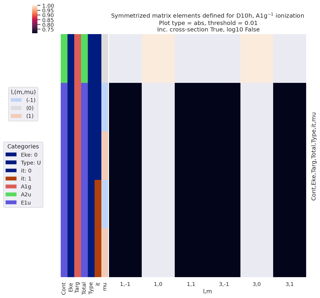
Fig. 6.4 Dipole-allowed continuum matrix elements for \(D_{10h}\), \(A_{1g}\) ionization, arranged by \((l,m)\).#
6.3.4.2. Mapping to fitting parameters (and reduction)#
Finally, the basis set of matrix elements can be assigned to a set of fitting parameters. In this case, as per Eq. (3.15), the parameters are mapped to magnitude-phase form; additionally, the fitting routine allows for the definition of relationships between the parameters. This provides a way to reduce the effective size of the basis set to only the unique values, with other terms defined purely by their symmetry relations. Consequently, degenerate cases, as detailed above, as well as cases with defined phase relations, can be efficiently reduced to a smaller basis set for fitting. Note that the default routine labels parameters by the full set of quantum numbers, with an m or p prefix to denote the magnitude and phase terms corresponding to the partial-wave channel; this ensures a unique naming scheme, but is also rather unwieldy (as can be seen below). In cases where fewer quantum numbers are required these can be defined and the parameter names remapped, see the PEMtk documentation [20] for further details.
For quick setup, there is an automated routine to set relations if applicable. The automated routine currently checks for the following relationships: identity (equal complex values), magnitude and phase equality, complex rotations by \(\pm\pi\), where matrix elements are grouped by symmetry (specifically Cont) and l prior to pair-wise testing. For more control, additional functions can be passed. Alternatively, the automatic setting can be skipped and/or relationships redefined or set manually. This provides a way to test if the symmetry-definitions are manifest in experimental data, rather than imposing them during fitting, or to explore other possible correlations between fitted parameters. Note, however, that in some cases the number of unique parameters in an unsymmetrized case may be large, so care should also be taken to ensure that fit results are meaningful in such cases (e.g. by employing a sufficiently large dataset, and testing for reproducibility).
# Default matrix element relationship tests are set by symCheckDefns
from pemtk.fit._sym import symCheckDefns

symCheckDefns()
{'i': {'name': 'identity',
  'lam': <function pemtk.fit._sym.symCheckDefns.<locals>.<lambda>(x)>,
  'transform': False,
  'constraint': 'x'},
 'abs': {'name': 'abs',
  'lam': <function pemtk.fit._sym.symCheckDefns.<locals>.<lambda>(x)>,
  'transform': True,
  'constraint': 'm_x'},
 'phase': {'name': 'phase',
  'lam': <function pemtk.fit._sym.symCheckDefns.<locals>.<lambda>(x)>,
  'transform': True,
  'constraint': 'p_x'},
 'crot_p': {'name': 'Complex rotation +pi/2',
  'lam': <function pemtk.fit._sym.symCheckDefns.<locals>.<lambda>(x)>,
  'transform': False,
  'constraint': 'arctan2(sin(p_x+pi/2), cos(p_x+pi/2))'},
 'crot_m': {'name': 'Complex rotation -pi/2',
  'lam': <function pemtk.fit._sym.symCheckDefns.<locals>.<lambda>(x)>,
  'transform': False,
  'constraint': 'arctan2(sin(p_x-pi/2), cos(p_x-pi/2))'}}
Automated assignment from defined matrix elements
The code blocks below illustrate the automated routine, and results are tabulated in Fig. 6.5.
from pemtk.fit.fitClass import pemtkFit

# Example using data class (setup in init script)
data = pemtkFit()

# Set to new key in data class
dataKey = sym
data.data[dataKey] = {}

# Assign allowed matrix elements to fit object
dataType = 'matE'
# General case - just use complex coeffs directly
# data.data[dataKey][dataType] = symObj.coeffs[dataType]['b (comp)']

# Specific case - e.g. sum over 'h'
data.data[dataKey][dataType] = symObjA1g.coeffs['symAllowed']['XR']['b (comp)'].sum('h')

# Propagate attrs
data.data[dataKey][dataType].attrs = symObjA1g.coeffs['symAllowed']['XR'].attrs
# Update selection with options
# E.g. Matrix element sub-selection
# data.selOpts['matE'] = {'thres': 0.01, 'inds': {'Type':'U','Cont':'A1'}}
data.selOpts['matE'] = {'thres': 0.01, 'inds': {'Type':'U'}}
data.setSubset(dataKey = sym, dataType = 'matE')  #, resetSelectors=True)  # Subselect from 'orb5' dataset, matrix elements

# And for the polarisation geometries...
# data.selOpts['pol'] = {'inds': {'Labels': 'z'}}
# data.setSubset(dataKey = 'pol', dataType = 'pol')
Subselected from dataset 'D10h', dataType 'matE': 72 from 540 points (13.33%)
# Set matrix elements to fitting parameters
# Running for the default case will attempt to automatically set the relations between
# matrix elements according to symmetry.
data.setMatEFit()
Show code cell output
Set 18 complex matrix elements to 36 fitting params, see self.params for details.
Auto-setting parameters.
| name | value | initial value | min | max | vary | expression |
|---|---|---|---|---|---|---|
| m_A2u_0_A1g_A2u_1_0_0_0 | 1.00000000 | 1.0 | 1.0000e-04 | 5.00000000 | True | |
| m_A2u_0_A1g_A2u_3_0_0_0 | 1.00000000 | 1.0 | 1.0000e-04 | 5.00000000 | True | |
| m_E1u_0_A1g_E1u_1_n1_n1_0 | 0.70710678 | 0.7071067811865475 | 1.0000e-04 | 5.00000000 | True | |
| m_E1u_0_A1g_E1u_1_n1_n1_1 | 0.70710678 | 0.7071067811865475 | 1.0000e-04 | 5.00000000 | True | |
| m_E1u_0_A1g_E1u_1_n1_1_0 | 0.70710678 | 0.7071067811865475 | 1.0000e-04 | 5.00000000 | False | m_E1u_0_A1g_E1u_1_n1_n1_0 |
| m_E1u_0_A1g_E1u_1_n1_1_1 | 0.70710678 | 0.7071067811865475 | 1.0000e-04 | 5.00000000 | False | m_E1u_0_A1g_E1u_1_n1_n1_0 |
| m_E1u_0_A1g_E1u_1_1_n1_0 | 0.70710678 | 0.7071067811865475 | 1.0000e-04 | 5.00000000 | False | m_E1u_0_A1g_E1u_1_n1_n1_0 |
| m_E1u_0_A1g_E1u_1_1_n1_1 | 0.70710678 | 0.7071067811865475 | 1.0000e-04 | 5.00000000 | False | m_E1u_0_A1g_E1u_1_n1_n1_0 |
| m_E1u_0_A1g_E1u_1_1_1_0 | 0.70710678 | 0.7071067811865475 | 1.0000e-04 | 5.00000000 | False | m_E1u_0_A1g_E1u_1_n1_n1_0 |
| m_E1u_0_A1g_E1u_1_1_1_1 | 0.70710678 | 0.7071067811865475 | 1.0000e-04 | 5.00000000 | False | m_E1u_0_A1g_E1u_1_n1_n1_0 |
| m_E1u_0_A1g_E1u_3_n1_n1_0 | 0.70710678 | 0.7071067811865475 | 1.0000e-04 | 5.00000000 | True | |
| m_E1u_0_A1g_E1u_3_n1_n1_1 | 0.70710678 | 0.7071067811865475 | 1.0000e-04 | 5.00000000 | True | |
| m_E1u_0_A1g_E1u_3_n1_1_0 | 0.70710678 | 0.7071067811865475 | 1.0000e-04 | 5.00000000 | False | m_E1u_0_A1g_E1u_3_n1_n1_0 |
| m_E1u_0_A1g_E1u_3_n1_1_1 | 0.70710678 | 0.7071067811865475 | 1.0000e-04 | 5.00000000 | False | m_E1u_0_A1g_E1u_3_n1_n1_0 |
| m_E1u_0_A1g_E1u_3_1_n1_0 | 0.70710678 | 0.7071067811865475 | 1.0000e-04 | 5.00000000 | False | m_E1u_0_A1g_E1u_3_n1_n1_0 |
| m_E1u_0_A1g_E1u_3_1_n1_1 | 0.70710678 | 0.7071067811865475 | 1.0000e-04 | 5.00000000 | False | m_E1u_0_A1g_E1u_3_n1_n1_0 |
| m_E1u_0_A1g_E1u_3_1_1_0 | 0.70710678 | 0.7071067811865475 | 1.0000e-04 | 5.00000000 | False | m_E1u_0_A1g_E1u_3_n1_n1_0 |
| m_E1u_0_A1g_E1u_3_1_1_1 | 0.70710678 | 0.7071067811865475 | 1.0000e-04 | 5.00000000 | False | m_E1u_0_A1g_E1u_3_n1_n1_0 |
| p_A2u_0_A1g_A2u_1_0_0_0 | 0.00000000 | 0.0 | -3.14159265 | 3.14159265 | False | |
| p_A2u_0_A1g_A2u_3_0_0_0 | 0.00000000 | 0.0 | -3.14159265 | 3.14159265 | True | |
| p_E1u_0_A1g_E1u_1_n1_n1_0 | 0.00000000 | 0.0 | -3.14159265 | 3.14159265 | True | |
| p_E1u_0_A1g_E1u_1_n1_n1_1 | 3.14159265 | 3.141592653589793 | -3.14159265 | 3.14159265 | True | |
| p_E1u_0_A1g_E1u_1_n1_1_0 | 0.00000000 | 0.0 | -3.14159265 | 3.14159265 | False | p_E1u_0_A1g_E1u_1_n1_n1_0 |
| p_E1u_0_A1g_E1u_1_n1_1_1 | 3.14159265 | 3.141592653589793 | -3.14159265 | 3.14159265 | False | p_E1u_0_A1g_E1u_1_n1_n1_1 |
| p_E1u_0_A1g_E1u_1_1_n1_0 | 3.14159265 | 3.141592653589793 | -3.14159265 | 3.14159265 | False | p_E1u_0_A1g_E1u_1_n1_n1_1 |
| p_E1u_0_A1g_E1u_1_1_n1_1 | 3.14159265 | 3.141592653589793 | -3.14159265 | 3.14159265 | False | p_E1u_0_A1g_E1u_1_n1_n1_1 |
| p_E1u_0_A1g_E1u_1_1_1_0 | 3.14159265 | 3.141592653589793 | -3.14159265 | 3.14159265 | False | p_E1u_0_A1g_E1u_1_n1_n1_1 |
| p_E1u_0_A1g_E1u_1_1_1_1 | 3.14159265 | 3.141592653589793 | -3.14159265 | 3.14159265 | False | p_E1u_0_A1g_E1u_1_n1_n1_1 |
| p_E1u_0_A1g_E1u_3_n1_n1_0 | 0.00000000 | 0.0 | -3.14159265 | 3.14159265 | True | |
| p_E1u_0_A1g_E1u_3_n1_n1_1 | 3.14159265 | 3.141592653589793 | -3.14159265 | 3.14159265 | True | |
| p_E1u_0_A1g_E1u_3_n1_1_0 | 0.00000000 | 0.0 | -3.14159265 | 3.14159265 | False | p_E1u_0_A1g_E1u_3_n1_n1_0 |
| p_E1u_0_A1g_E1u_3_n1_1_1 | 3.14159265 | 3.141592653589793 | -3.14159265 | 3.14159265 | False | p_E1u_0_A1g_E1u_3_n1_n1_1 |
| p_E1u_0_A1g_E1u_3_1_n1_0 | 3.14159265 | 3.141592653589793 | -3.14159265 | 3.14159265 | False | p_E1u_0_A1g_E1u_3_n1_n1_1 |
| p_E1u_0_A1g_E1u_3_1_n1_1 | 3.14159265 | 3.141592653589793 | -3.14159265 | 3.14159265 | False | p_E1u_0_A1g_E1u_3_n1_n1_1 |
| p_E1u_0_A1g_E1u_3_1_1_0 | 3.14159265 | 3.141592653589793 | -3.14159265 | 3.14159265 | False | p_E1u_0_A1g_E1u_3_n1_n1_1 |
| p_E1u_0_A1g_E1u_3_1_1_1 | 3.14159265 | 3.141592653589793 | -3.14159265 | 3.14159265 | False | p_E1u_0_A1g_E1u_3_n1_n1_1 |
Show code cell content
# Glue table for later
# Need wrapper here otherwise get plain text in current HTML builds, and print(data.params) in PDF version (no data.params._repr_latex_())
glue("fittingParamsD10hA1g", params_to_dataframe(data.params))

# display(data.params)
| name | value | stderr | vary | expr | init_value | min | max | brute_step | correl | |
|---|---|---|---|---|---|---|---|---|---|---|
| 0 | m_A2u_0_A1g_A2u_1_0_0_0 | 1.000 | None | True | None | 1.000 | 1.000e-04 | 5.000 | None | None |
| 1 | m_A2u_0_A1g_A2u_3_0_0_0 | 1.000 | None | True | None | 1.000 | 1.000e-04 | 5.000 | None | None |
| 2 | m_E1u_0_A1g_E1u_1_n1_n1_0 | 0.707 | None | True | None | 0.707 | 1.000e-04 | 5.000 | None | None |
| 3 | m_E1u_0_A1g_E1u_1_n1_n1_1 | 0.707 | None | True | None | 0.707 | 1.000e-04 | 5.000 | None | None |
| 4 | m_E1u_0_A1g_E1u_1_n1_1_0 | 0.707 | None | False | m_E1u_0_A1g_E1u_1_n1_n1_0 | 0.707 | 1.000e-04 | 5.000 | None | None |
| 5 | m_E1u_0_A1g_E1u_1_n1_1_1 | 0.707 | None | False | m_E1u_0_A1g_E1u_1_n1_n1_0 | 0.707 | 1.000e-04 | 5.000 | None | None |
| 6 | m_E1u_0_A1g_E1u_1_1_n1_0 | 0.707 | None | False | m_E1u_0_A1g_E1u_1_n1_n1_0 | 0.707 | 1.000e-04 | 5.000 | None | None |
| 7 | m_E1u_0_A1g_E1u_1_1_n1_1 | 0.707 | None | False | m_E1u_0_A1g_E1u_1_n1_n1_0 | 0.707 | 1.000e-04 | 5.000 | None | None |
| 8 | m_E1u_0_A1g_E1u_1_1_1_0 | 0.707 | None | False | m_E1u_0_A1g_E1u_1_n1_n1_0 | 0.707 | 1.000e-04 | 5.000 | None | None |
| 9 | m_E1u_0_A1g_E1u_1_1_1_1 | 0.707 | None | False | m_E1u_0_A1g_E1u_1_n1_n1_0 | 0.707 | 1.000e-04 | 5.000 | None | None |
| 10 | m_E1u_0_A1g_E1u_3_n1_n1_0 | 0.707 | None | True | None | 0.707 | 1.000e-04 | 5.000 | None | None |
| 11 | m_E1u_0_A1g_E1u_3_n1_n1_1 | 0.707 | None | True | None | 0.707 | 1.000e-04 | 5.000 | None | None |
| 12 | m_E1u_0_A1g_E1u_3_n1_1_0 | 0.707 | None | False | m_E1u_0_A1g_E1u_3_n1_n1_0 | 0.707 | 1.000e-04 | 5.000 | None | None |
| 13 | m_E1u_0_A1g_E1u_3_n1_1_1 | 0.707 | None | False | m_E1u_0_A1g_E1u_3_n1_n1_0 | 0.707 | 1.000e-04 | 5.000 | None | None |
| 14 | m_E1u_0_A1g_E1u_3_1_n1_0 | 0.707 | None | False | m_E1u_0_A1g_E1u_3_n1_n1_0 | 0.707 | 1.000e-04 | 5.000 | None | None |
| 15 | m_E1u_0_A1g_E1u_3_1_n1_1 | 0.707 | None | False | m_E1u_0_A1g_E1u_3_n1_n1_0 | 0.707 | 1.000e-04 | 5.000 | None | None |
| 16 | m_E1u_0_A1g_E1u_3_1_1_0 | 0.707 | None | False | m_E1u_0_A1g_E1u_3_n1_n1_0 | 0.707 | 1.000e-04 | 5.000 | None | None |
| 17 | m_E1u_0_A1g_E1u_3_1_1_1 | 0.707 | None | False | m_E1u_0_A1g_E1u_3_n1_n1_0 | 0.707 | 1.000e-04 | 5.000 | None | None |
| 18 | p_A2u_0_A1g_A2u_1_0_0_0 | 0.000 | None | False | None | 0.000 | -3.142e+00 | 3.142 | None | None |
| 19 | p_A2u_0_A1g_A2u_3_0_0_0 | 0.000 | None | True | None | 0.000 | -3.142e+00 | 3.142 | None | None |
| 20 | p_E1u_0_A1g_E1u_1_n1_n1_0 | 0.000 | None | True | None | 0.000 | -3.142e+00 | 3.142 | None | None |
| 21 | p_E1u_0_A1g_E1u_1_n1_n1_1 | 3.142 | None | True | None | 3.142 | -3.142e+00 | 3.142 | None | None |
| 22 | p_E1u_0_A1g_E1u_1_n1_1_0 | 0.000 | None | False | p_E1u_0_A1g_E1u_1_n1_n1_0 | 0.000 | -3.142e+00 | 3.142 | None | None |
| 23 | p_E1u_0_A1g_E1u_1_n1_1_1 | 3.142 | None | False | p_E1u_0_A1g_E1u_1_n1_n1_1 | 3.142 | -3.142e+00 | 3.142 | None | None |
| 24 | p_E1u_0_A1g_E1u_1_1_n1_0 | 3.142 | None | False | p_E1u_0_A1g_E1u_1_n1_n1_1 | 3.142 | -3.142e+00 | 3.142 | None | None |
| 25 | p_E1u_0_A1g_E1u_1_1_n1_1 | 3.142 | None | False | p_E1u_0_A1g_E1u_1_n1_n1_1 | 3.142 | -3.142e+00 | 3.142 | None | None |
| 26 | p_E1u_0_A1g_E1u_1_1_1_0 | 3.142 | None | False | p_E1u_0_A1g_E1u_1_n1_n1_1 | 3.142 | -3.142e+00 | 3.142 | None | None |
| 27 | p_E1u_0_A1g_E1u_1_1_1_1 | 3.142 | None | False | p_E1u_0_A1g_E1u_1_n1_n1_1 | 3.142 | -3.142e+00 | 3.142 | None | None |
| 28 | p_E1u_0_A1g_E1u_3_n1_n1_0 | 0.000 | None | True | None | 0.000 | -3.142e+00 | 3.142 | None | None |
| 29 | p_E1u_0_A1g_E1u_3_n1_n1_1 | 3.142 | None | True | None | 3.142 | -3.142e+00 | 3.142 | None | None |
| 30 | p_E1u_0_A1g_E1u_3_n1_1_0 | 0.000 | None | False | p_E1u_0_A1g_E1u_3_n1_n1_0 | 0.000 | -3.142e+00 | 3.142 | None | None |
| 31 | p_E1u_0_A1g_E1u_3_n1_1_1 | 3.142 | None | False | p_E1u_0_A1g_E1u_3_n1_n1_1 | 3.142 | -3.142e+00 | 3.142 | None | None |
| 32 | p_E1u_0_A1g_E1u_3_1_n1_0 | 3.142 | None | False | p_E1u_0_A1g_E1u_3_n1_n1_1 | 3.142 | -3.142e+00 | 3.142 | None | None |
| 33 | p_E1u_0_A1g_E1u_3_1_n1_1 | 3.142 | None | False | p_E1u_0_A1g_E1u_3_n1_n1_1 | 3.142 | -3.142e+00 | 3.142 | None | None |
| 34 | p_E1u_0_A1g_E1u_3_1_1_0 | 3.142 | None | False | p_E1u_0_A1g_E1u_3_n1_n1_1 | 3.142 | -3.142e+00 | 3.142 | None | None |
| 35 | p_E1u_0_A1g_E1u_3_1_1_1 | 3.142 | None | False | p_E1u_0_A1g_E1u_3_n1_n1_1 | 3.142 | -3.142e+00 | 3.142 | None | None |
Fig. 6.5 Fitting parameters as assigned for \(D_{10h}\), \(A_{1g}\) ionization. Note the vary column, which defines the symmetry-unique values for fitting, whilst the expression column indicates the relationships of the non-unique values to the floated parameters.#
Modifying fitting basis parameters
A brief illustration of defining constraints is given below, for more details see the PEMtk documentation [20], particularly the basic fitting guide. For more details on the base lmfit parameters class that is used here, see lmfit library [66, 67], particularly the documentation on parameters and constraints.
# Set parameters with NO constraints set (except a reference phase)
data.setMatEFit(paramsCons = None)
Show code cell output
Set 18 complex matrix elements to 36 fitting params, see self.params for details.
| name | value | initial value | min | max | vary |
|---|---|---|---|---|---|
| m_A2u_0_A1g_A2u_1_0_0_0 | 1.00000000 | 1.0 | 1.0000e-04 | 5.00000000 | True |
| m_A2u_0_A1g_A2u_3_0_0_0 | 1.00000000 | 1.0 | 1.0000e-04 | 5.00000000 | True |
| m_E1u_0_A1g_E1u_1_n1_n1_0 | 0.70710678 | 0.7071067811865475 | 1.0000e-04 | 5.00000000 | True |
| m_E1u_0_A1g_E1u_1_n1_n1_1 | 0.70710678 | 0.7071067811865475 | 1.0000e-04 | 5.00000000 | True |
| m_E1u_0_A1g_E1u_1_n1_1_0 | 0.70710678 | 0.7071067811865475 | 1.0000e-04 | 5.00000000 | True |
| m_E1u_0_A1g_E1u_1_n1_1_1 | 0.70710678 | 0.7071067811865475 | 1.0000e-04 | 5.00000000 | True |
| m_E1u_0_A1g_E1u_1_1_n1_0 | 0.70710678 | 0.7071067811865475 | 1.0000e-04 | 5.00000000 | True |
| m_E1u_0_A1g_E1u_1_1_n1_1 | 0.70710678 | 0.7071067811865475 | 1.0000e-04 | 5.00000000 | True |
| m_E1u_0_A1g_E1u_1_1_1_0 | 0.70710678 | 0.7071067811865475 | 1.0000e-04 | 5.00000000 | True |
| m_E1u_0_A1g_E1u_1_1_1_1 | 0.70710678 | 0.7071067811865475 | 1.0000e-04 | 5.00000000 | True |
| m_E1u_0_A1g_E1u_3_n1_n1_0 | 0.70710678 | 0.7071067811865475 | 1.0000e-04 | 5.00000000 | True |
| m_E1u_0_A1g_E1u_3_n1_n1_1 | 0.70710678 | 0.7071067811865475 | 1.0000e-04 | 5.00000000 | True |
| m_E1u_0_A1g_E1u_3_n1_1_0 | 0.70710678 | 0.7071067811865475 | 1.0000e-04 | 5.00000000 | True |
| m_E1u_0_A1g_E1u_3_n1_1_1 | 0.70710678 | 0.7071067811865475 | 1.0000e-04 | 5.00000000 | True |
| m_E1u_0_A1g_E1u_3_1_n1_0 | 0.70710678 | 0.7071067811865475 | 1.0000e-04 | 5.00000000 | True |
| m_E1u_0_A1g_E1u_3_1_n1_1 | 0.70710678 | 0.7071067811865475 | 1.0000e-04 | 5.00000000 | True |
| m_E1u_0_A1g_E1u_3_1_1_0 | 0.70710678 | 0.7071067811865475 | 1.0000e-04 | 5.00000000 | True |
| m_E1u_0_A1g_E1u_3_1_1_1 | 0.70710678 | 0.7071067811865475 | 1.0000e-04 | 5.00000000 | True |
| p_A2u_0_A1g_A2u_1_0_0_0 | 0.00000000 | 0.0 | -3.14159265 | 3.14159265 | False |
| p_A2u_0_A1g_A2u_3_0_0_0 | 0.00000000 | 0.0 | -3.14159265 | 3.14159265 | True |
| p_E1u_0_A1g_E1u_1_n1_n1_0 | 0.00000000 | 0.0 | -3.14159265 | 3.14159265 | True |
| p_E1u_0_A1g_E1u_1_n1_n1_1 | 3.14159265 | 3.141592653589793 | -3.14159265 | 3.14159265 | True |
| p_E1u_0_A1g_E1u_1_n1_1_0 | 0.00000000 | 0.0 | -3.14159265 | 3.14159265 | True |
| p_E1u_0_A1g_E1u_1_n1_1_1 | 3.14159265 | 3.141592653589793 | -3.14159265 | 3.14159265 | True |
| p_E1u_0_A1g_E1u_1_1_n1_0 | 3.14159265 | 3.141592653589793 | -3.14159265 | 3.14159265 | True |
| p_E1u_0_A1g_E1u_1_1_n1_1 | 3.14159265 | 3.141592653589793 | -3.14159265 | 3.14159265 | True |
| p_E1u_0_A1g_E1u_1_1_1_0 | 3.14159265 | 3.141592653589793 | -3.14159265 | 3.14159265 | True |
| p_E1u_0_A1g_E1u_1_1_1_1 | 3.14159265 | 3.141592653589793 | -3.14159265 | 3.14159265 | True |
| p_E1u_0_A1g_E1u_3_n1_n1_0 | 0.00000000 | 0.0 | -3.14159265 | 3.14159265 | True |
| p_E1u_0_A1g_E1u_3_n1_n1_1 | 3.14159265 | 3.141592653589793 | -3.14159265 | 3.14159265 | True |
| p_E1u_0_A1g_E1u_3_n1_1_0 | 0.00000000 | 0.0 | -3.14159265 | 3.14159265 | True |
| p_E1u_0_A1g_E1u_3_n1_1_1 | 3.14159265 | 3.141592653589793 | -3.14159265 | 3.14159265 | True |
| p_E1u_0_A1g_E1u_3_1_n1_0 | 3.14159265 | 3.141592653589793 | -3.14159265 | 3.14159265 | True |
| p_E1u_0_A1g_E1u_3_1_n1_1 | 3.14159265 | 3.141592653589793 | -3.14159265 | 3.14159265 | True |
| p_E1u_0_A1g_E1u_3_1_1_0 | 3.14159265 | 3.141592653589793 | -3.14159265 | 3.14159265 | True |
| p_E1u_0_A1g_E1u_3_1_1_1 | 3.14159265 | 3.141592653589793 | -3.14159265 | 3.14159265 | True |
# To add manual constraints
# Set param constraints as dict
# Any basic mathematical relations can be set here,
# see https://lmfit.github.io/lmfit-py/constraints.html
paramsCons = {}
paramsCons['m_A2u_0_A1g_A2u_1_0_0_0'] = '5*m_A2u_0_A1g_A2u_3_0_0_0'

# Missing settings will generate an error message
paramsCons['test'] = 'p_PU_SG_PU_3_1_n1_1'

# Init parameters with specified constraints
data.setMatEFit(paramsCons = paramsCons)
Show code cell output
Set 18 complex matrix elements to 36 fitting params, see self.params for details.
*** Warning, parameter test not present, skipping constraint test = p_PU_SG_PU_3_1_n1_1
| name | value | initial value | min | max | vary | expression |
|---|---|---|---|---|---|---|
| m_A2u_0_A1g_A2u_1_0_0_0 | 5.00000000 | 1.0 | 1.0000e-04 | 5.00000000 | False | 5*m_A2u_0_A1g_A2u_3_0_0_0 |
| m_A2u_0_A1g_A2u_3_0_0_0 | 1.00000000 | 1.0 | 1.0000e-04 | 5.00000000 | True | |
| m_E1u_0_A1g_E1u_1_n1_n1_0 | 0.70710678 | 0.7071067811865475 | 1.0000e-04 | 5.00000000 | True | |
| m_E1u_0_A1g_E1u_1_n1_n1_1 | 0.70710678 | 0.7071067811865475 | 1.0000e-04 | 5.00000000 | True | |
| m_E1u_0_A1g_E1u_1_n1_1_0 | 0.70710678 | 0.7071067811865475 | 1.0000e-04 | 5.00000000 | True | |
| m_E1u_0_A1g_E1u_1_n1_1_1 | 0.70710678 | 0.7071067811865475 | 1.0000e-04 | 5.00000000 | True | |
| m_E1u_0_A1g_E1u_1_1_n1_0 | 0.70710678 | 0.7071067811865475 | 1.0000e-04 | 5.00000000 | True | |
| m_E1u_0_A1g_E1u_1_1_n1_1 | 0.70710678 | 0.7071067811865475 | 1.0000e-04 | 5.00000000 | True | |
| m_E1u_0_A1g_E1u_1_1_1_0 | 0.70710678 | 0.7071067811865475 | 1.0000e-04 | 5.00000000 | True | |
| m_E1u_0_A1g_E1u_1_1_1_1 | 0.70710678 | 0.7071067811865475 | 1.0000e-04 | 5.00000000 | True | |
| m_E1u_0_A1g_E1u_3_n1_n1_0 | 0.70710678 | 0.7071067811865475 | 1.0000e-04 | 5.00000000 | True | |
| m_E1u_0_A1g_E1u_3_n1_n1_1 | 0.70710678 | 0.7071067811865475 | 1.0000e-04 | 5.00000000 | True | |
| m_E1u_0_A1g_E1u_3_n1_1_0 | 0.70710678 | 0.7071067811865475 | 1.0000e-04 | 5.00000000 | True | |
| m_E1u_0_A1g_E1u_3_n1_1_1 | 0.70710678 | 0.7071067811865475 | 1.0000e-04 | 5.00000000 | True | |
| m_E1u_0_A1g_E1u_3_1_n1_0 | 0.70710678 | 0.7071067811865475 | 1.0000e-04 | 5.00000000 | True | |
| m_E1u_0_A1g_E1u_3_1_n1_1 | 0.70710678 | 0.7071067811865475 | 1.0000e-04 | 5.00000000 | True | |
| m_E1u_0_A1g_E1u_3_1_1_0 | 0.70710678 | 0.7071067811865475 | 1.0000e-04 | 5.00000000 | True | |
| m_E1u_0_A1g_E1u_3_1_1_1 | 0.70710678 | 0.7071067811865475 | 1.0000e-04 | 5.00000000 | True | |
| p_A2u_0_A1g_A2u_1_0_0_0 | 0.00000000 | 0.0 | -3.14159265 | 3.14159265 | False | |
| p_A2u_0_A1g_A2u_3_0_0_0 | 0.00000000 | 0.0 | -3.14159265 | 3.14159265 | True | |
| p_E1u_0_A1g_E1u_1_n1_n1_0 | 0.00000000 | 0.0 | -3.14159265 | 3.14159265 | True | |
| p_E1u_0_A1g_E1u_1_n1_n1_1 | 3.14159265 | 3.141592653589793 | -3.14159265 | 3.14159265 | True | |
| p_E1u_0_A1g_E1u_1_n1_1_0 | 0.00000000 | 0.0 | -3.14159265 | 3.14159265 | True | |
| p_E1u_0_A1g_E1u_1_n1_1_1 | 3.14159265 | 3.141592653589793 | -3.14159265 | 3.14159265 | True | |
| p_E1u_0_A1g_E1u_1_1_n1_0 | 3.14159265 | 3.141592653589793 | -3.14159265 | 3.14159265 | True | |
| p_E1u_0_A1g_E1u_1_1_n1_1 | 3.14159265 | 3.141592653589793 | -3.14159265 | 3.14159265 | True | |
| p_E1u_0_A1g_E1u_1_1_1_0 | 3.14159265 | 3.141592653589793 | -3.14159265 | 3.14159265 | True | |
| p_E1u_0_A1g_E1u_1_1_1_1 | 3.14159265 | 3.141592653589793 | -3.14159265 | 3.14159265 | True | |
| p_E1u_0_A1g_E1u_3_n1_n1_0 | 0.00000000 | 0.0 | -3.14159265 | 3.14159265 | True | |
| p_E1u_0_A1g_E1u_3_n1_n1_1 | 3.14159265 | 3.141592653589793 | -3.14159265 | 3.14159265 | True | |
| p_E1u_0_A1g_E1u_3_n1_1_0 | 0.00000000 | 0.0 | -3.14159265 | 3.14159265 | True | |
| p_E1u_0_A1g_E1u_3_n1_1_1 | 3.14159265 | 3.141592653589793 | -3.14159265 | 3.14159265 | True | |
| p_E1u_0_A1g_E1u_3_1_n1_0 | 3.14159265 | 3.141592653589793 | -3.14159265 | 3.14159265 | True | |
| p_E1u_0_A1g_E1u_3_1_n1_1 | 3.14159265 | 3.141592653589793 | -3.14159265 | 3.14159265 | True | |
| p_E1u_0_A1g_E1u_3_1_1_0 | 3.14159265 | 3.141592653589793 | -3.14159265 | 3.14159265 | True | |
| p_E1u_0_A1g_E1u_3_1_1_1 | 3.14159265 | 3.141592653589793 | -3.14159265 | 3.14159265 | True |
# Individual parameters can be addressed by name,

data.params['m_E1u_0_A1g_E1u_1_n1_n1_0']
<Parameter 'm_E1u_0_A1g_E1u_1_n1_n1_0', value=0.7071067811865475, bounds=[0.0001:5.0]>
# Properties can be modified directly...
data.params['m_A2u_0_A1g_A2u_3_0_0_0'].value = 1.777

# ...or by using lmfit's `.set()` method.
data.params['m_E1u_0_A1g_E1u_1_n1_n1_0'].set(value = 1.36)
data.params['m_E1u_0_A1g_E1u_1_n1_n1_0'].set(vary = False)
data.params['m_E1u_0_A1g_E1u_1_n1_n1_0']
<Parameter 'm_E1u_0_A1g_E1u_1_n1_n1_0', value=1.36 (fixed), bounds=[0.0001:5.0]>
# The full set can always be checked via self.params
data.params
Show code cell output
| name | value | initial value | min | max | vary | expression |
|---|---|---|---|---|---|---|
| m_A2u_0_A1g_A2u_1_0_0_0 | 5.00000000 | 1.0 | 1.0000e-04 | 5.00000000 | False | 5*m_A2u_0_A1g_A2u_3_0_0_0 |
| m_A2u_0_A1g_A2u_3_0_0_0 | 1.77700000 | 1.0 | 1.0000e-04 | 5.00000000 | True | |
| m_E1u_0_A1g_E1u_1_n1_n1_0 | 1.36000000 | 1.36 | 1.0000e-04 | 5.00000000 | False | |
| m_E1u_0_A1g_E1u_1_n1_n1_1 | 0.70710678 | 0.7071067811865475 | 1.0000e-04 | 5.00000000 | True | |
| m_E1u_0_A1g_E1u_1_n1_1_0 | 0.70710678 | 0.7071067811865475 | 1.0000e-04 | 5.00000000 | True | |
| m_E1u_0_A1g_E1u_1_n1_1_1 | 0.70710678 | 0.7071067811865475 | 1.0000e-04 | 5.00000000 | True | |
| m_E1u_0_A1g_E1u_1_1_n1_0 | 0.70710678 | 0.7071067811865475 | 1.0000e-04 | 5.00000000 | True | |
| m_E1u_0_A1g_E1u_1_1_n1_1 | 0.70710678 | 0.7071067811865475 | 1.0000e-04 | 5.00000000 | True | |
| m_E1u_0_A1g_E1u_1_1_1_0 | 0.70710678 | 0.7071067811865475 | 1.0000e-04 | 5.00000000 | True | |
| m_E1u_0_A1g_E1u_1_1_1_1 | 0.70710678 | 0.7071067811865475 | 1.0000e-04 | 5.00000000 | True | |
| m_E1u_0_A1g_E1u_3_n1_n1_0 | 0.70710678 | 0.7071067811865475 | 1.0000e-04 | 5.00000000 | True | |
| m_E1u_0_A1g_E1u_3_n1_n1_1 | 0.70710678 | 0.7071067811865475 | 1.0000e-04 | 5.00000000 | True | |
| m_E1u_0_A1g_E1u_3_n1_1_0 | 0.70710678 | 0.7071067811865475 | 1.0000e-04 | 5.00000000 | True | |
| m_E1u_0_A1g_E1u_3_n1_1_1 | 0.70710678 | 0.7071067811865475 | 1.0000e-04 | 5.00000000 | True | |
| m_E1u_0_A1g_E1u_3_1_n1_0 | 0.70710678 | 0.7071067811865475 | 1.0000e-04 | 5.00000000 | True | |
| m_E1u_0_A1g_E1u_3_1_n1_1 | 0.70710678 | 0.7071067811865475 | 1.0000e-04 | 5.00000000 | True | |
| m_E1u_0_A1g_E1u_3_1_1_0 | 0.70710678 | 0.7071067811865475 | 1.0000e-04 | 5.00000000 | True | |
| m_E1u_0_A1g_E1u_3_1_1_1 | 0.70710678 | 0.7071067811865475 | 1.0000e-04 | 5.00000000 | True | |
| p_A2u_0_A1g_A2u_1_0_0_0 | 0.00000000 | 0.0 | -3.14159265 | 3.14159265 | False | |
| p_A2u_0_A1g_A2u_3_0_0_0 | 0.00000000 | 0.0 | -3.14159265 | 3.14159265 | True | |
| p_E1u_0_A1g_E1u_1_n1_n1_0 | 0.00000000 | 0.0 | -3.14159265 | 3.14159265 | True | |
| p_E1u_0_A1g_E1u_1_n1_n1_1 | 3.14159265 | 3.141592653589793 | -3.14159265 | 3.14159265 | True | |
| p_E1u_0_A1g_E1u_1_n1_1_0 | 0.00000000 | 0.0 | -3.14159265 | 3.14159265 | True | |
| p_E1u_0_A1g_E1u_1_n1_1_1 | 3.14159265 | 3.141592653589793 | -3.14159265 | 3.14159265 | True | |
| p_E1u_0_A1g_E1u_1_1_n1_0 | 3.14159265 | 3.141592653589793 | -3.14159265 | 3.14159265 | True | |
| p_E1u_0_A1g_E1u_1_1_n1_1 | 3.14159265 | 3.141592653589793 | -3.14159265 | 3.14159265 | True | |
| p_E1u_0_A1g_E1u_1_1_1_0 | 3.14159265 | 3.141592653589793 | -3.14159265 | 3.14159265 | True | |
| p_E1u_0_A1g_E1u_1_1_1_1 | 3.14159265 | 3.141592653589793 | -3.14159265 | 3.14159265 | True | |
| p_E1u_0_A1g_E1u_3_n1_n1_0 | 0.00000000 | 0.0 | -3.14159265 | 3.14159265 | True | |
| p_E1u_0_A1g_E1u_3_n1_n1_1 | 3.14159265 | 3.141592653589793 | -3.14159265 | 3.14159265 | True | |
| p_E1u_0_A1g_E1u_3_n1_1_0 | 0.00000000 | 0.0 | -3.14159265 | 3.14159265 | True | |
| p_E1u_0_A1g_E1u_3_n1_1_1 | 3.14159265 | 3.141592653589793 | -3.14159265 | 3.14159265 | True | |
| p_E1u_0_A1g_E1u_3_1_n1_0 | 3.14159265 | 3.141592653589793 | -3.14159265 | 3.14159265 | True | |
| p_E1u_0_A1g_E1u_3_1_n1_1 | 3.14159265 | 3.141592653589793 | -3.14159265 | 3.14159265 | True | |
| p_E1u_0_A1g_E1u_3_1_1_0 | 3.14159265 | 3.141592653589793 | -3.14159265 | 3.14159265 | True | |
| p_E1u_0_A1g_E1u_3_1_1_1 | 3.14159265 | 3.141592653589793 | -3.14159265 | 3.14159265 | True |
# The full mapping of parameter names and indexes is given in self.lmmu
data.lmmu
Show code cell output
{'Index': MultiIndex([('A2u', 0, 'A1g', 'A2u', 1,  0,  0, 0),
             ('A2u', 0, 'A1g', 'A2u', 3,  0,  0, 0),
             ('E1u', 0, 'A1g', 'E1u', 1, -1, -1, 0),
             ('E1u', 0, 'A1g', 'E1u', 1, -1, -1, 1),
             ('E1u', 0, 'A1g', 'E1u', 1, -1,  1, 0),
             ('E1u', 0, 'A1g', 'E1u', 1, -1,  1, 1),
             ('E1u', 0, 'A1g', 'E1u', 1,  1, -1, 0),
             ('E1u', 0, 'A1g', 'E1u', 1,  1, -1, 1),
             ('E1u', 0, 'A1g', 'E1u', 1,  1,  1, 0),
             ('E1u', 0, 'A1g', 'E1u', 1,  1,  1, 1),
             ('E1u', 0, 'A1g', 'E1u', 3, -1, -1, 0),
             ('E1u', 0, 'A1g', 'E1u', 3, -1, -1, 1),
             ('E1u', 0, 'A1g', 'E1u', 3, -1,  1, 0),
             ('E1u', 0, 'A1g', 'E1u', 3, -1,  1, 1),
             ('E1u', 0, 'A1g', 'E1u', 3,  1, -1, 0),
             ('E1u', 0, 'A1g', 'E1u', 3,  1, -1, 1),
             ('E1u', 0, 'A1g', 'E1u', 3,  1,  1, 0),
             ('E1u', 0, 'A1g', 'E1u', 3,  1,  1, 1)],
            names=['Cont', 'Eke', 'Targ', 'Total', 'l', 'm', 'mu', 'it']),
 'Str': ['A2u_0_A1g_A2u_1_0_0_0',
  'A2u_0_A1g_A2u_3_0_0_0',
  'E1u_0_A1g_E1u_1_n1_n1_0',
  'E1u_0_A1g_E1u_1_n1_n1_1',
  'E1u_0_A1g_E1u_1_n1_1_0',
  'E1u_0_A1g_E1u_1_n1_1_1',
  'E1u_0_A1g_E1u_1_1_n1_0',
  'E1u_0_A1g_E1u_1_1_n1_1',
  'E1u_0_A1g_E1u_1_1_1_0',
  'E1u_0_A1g_E1u_1_1_1_1',
  'E1u_0_A1g_E1u_3_n1_n1_0',
  'E1u_0_A1g_E1u_3_n1_n1_1',
  'E1u_0_A1g_E1u_3_n1_1_0',
  'E1u_0_A1g_E1u_3_n1_1_1',
  'E1u_0_A1g_E1u_3_1_n1_0',
  'E1u_0_A1g_E1u_3_1_n1_1',
  'E1u_0_A1g_E1u_3_1_1_0',
  'E1u_0_A1g_E1u_3_1_1_1'],
 'lmMap': {'A2u_0_A1g_A2u_1_0_0_0': '0,1,0',
  'A2u_0_A1g_A2u_3_0_0_0': '0,3,0',
  'E1u_0_A1g_E1u_1_n1_n1_0': '0,1,-1',
  'E1u_0_A1g_E1u_1_n1_n1_1': '0,1,-1',
  'E1u_0_A1g_E1u_1_n1_1_0': '0,1,-1',
  'E1u_0_A1g_E1u_1_n1_1_1': '0,1,-1',
  'E1u_0_A1g_E1u_1_1_n1_0': '0,1,1',
  'E1u_0_A1g_E1u_1_1_n1_1': '0,1,1',
  'E1u_0_A1g_E1u_1_1_1_0': '0,1,1',
  'E1u_0_A1g_E1u_1_1_1_1': '0,1,1',
  'E1u_0_A1g_E1u_3_n1_n1_0': '0,3,-1',
  'E1u_0_A1g_E1u_3_n1_n1_1': '0,3,-1',
  'E1u_0_A1g_E1u_3_n1_1_0': '0,3,-1',
  'E1u_0_A1g_E1u_3_n1_1_1': '0,3,-1',
  'E1u_0_A1g_E1u_3_1_n1_0': '0,3,1',
  'E1u_0_A1g_E1u_3_1_n1_1': '0,3,1',
  'E1u_0_A1g_E1u_3_1_1_0': '0,3,1',
  'E1u_0_A1g_E1u_3_1_1_1': '0,3,1'},
 'map': [('A2u_0_A1g_A2u_1_0_0_0',
   [0, 18],
   'm_A2u_0_A1g_A2u_1_0_0_0',
   'p_A2u_0_A1g_A2u_1_0_0_0'),
  ('A2u_0_A1g_A2u_3_0_0_0',
   [1, 19],
   'm_A2u_0_A1g_A2u_3_0_0_0',
   'p_A2u_0_A1g_A2u_3_0_0_0'),
  ('E1u_0_A1g_E1u_1_n1_n1_0',
   [2, 20],
   'm_E1u_0_A1g_E1u_1_n1_n1_0',
   'p_E1u_0_A1g_E1u_1_n1_n1_0'),
  ('E1u_0_A1g_E1u_1_n1_n1_1',
   [3, 21],
   'm_E1u_0_A1g_E1u_1_n1_n1_1',
   'p_E1u_0_A1g_E1u_1_n1_n1_1'),
  ('E1u_0_A1g_E1u_1_n1_1_0',
   [4, 22],
   'm_E1u_0_A1g_E1u_1_n1_1_0',
   'p_E1u_0_A1g_E1u_1_n1_1_0'),
  ('E1u_0_A1g_E1u_1_n1_1_1',
   [5, 23],
   'm_E1u_0_A1g_E1u_1_n1_1_1',
   'p_E1u_0_A1g_E1u_1_n1_1_1'),
  ('E1u_0_A1g_E1u_1_1_n1_0',
   [6, 24],
   'm_E1u_0_A1g_E1u_1_1_n1_0',
   'p_E1u_0_A1g_E1u_1_1_n1_0'),
  ('E1u_0_A1g_E1u_1_1_n1_1',
   [7, 25],
   'm_E1u_0_A1g_E1u_1_1_n1_1',
   'p_E1u_0_A1g_E1u_1_1_n1_1'),
  ('E1u_0_A1g_E1u_1_1_1_0',
   [8, 26],
   'm_E1u_0_A1g_E1u_1_1_1_0',
   'p_E1u_0_A1g_E1u_1_1_1_0'),
  ('E1u_0_A1g_E1u_1_1_1_1',
   [9, 27],
   'm_E1u_0_A1g_E1u_1_1_1_1',
   'p_E1u_0_A1g_E1u_1_1_1_1'),
  ('E1u_0_A1g_E1u_3_n1_n1_0',
   [10, 28],
   'm_E1u_0_A1g_E1u_3_n1_n1_0',
   'p_E1u_0_A1g_E1u_3_n1_n1_0'),
  ('E1u_0_A1g_E1u_3_n1_n1_1',
   [11, 29],
   'm_E1u_0_A1g_E1u_3_n1_n1_1',
   'p_E1u_0_A1g_E1u_3_n1_n1_1'),
  ('E1u_0_A1g_E1u_3_n1_1_0',
   [12, 30],
   'm_E1u_0_A1g_E1u_3_n1_1_0',
   'p_E1u_0_A1g_E1u_3_n1_1_0'),
  ('E1u_0_A1g_E1u_3_n1_1_1',
   [13, 31],
   'm_E1u_0_A1g_E1u_3_n1_1_1',
   'p_E1u_0_A1g_E1u_3_n1_1_1'),
  ('E1u_0_A1g_E1u_3_1_n1_0',
   [14, 32],
   'm_E1u_0_A1g_E1u_3_1_n1_0',
   'p_E1u_0_A1g_E1u_3_1_n1_0'),
  ('E1u_0_A1g_E1u_3_1_n1_1',
   [15, 33],
   'm_E1u_0_A1g_E1u_3_1_n1_1',
   'p_E1u_0_A1g_E1u_3_1_n1_1'),
  ('E1u_0_A1g_E1u_3_1_1_0',
   [16, 34],
   'm_E1u_0_A1g_E1u_3_1_1_0',
   'p_E1u_0_A1g_E1u_3_1_1_0'),
  ('E1u_0_A1g_E1u_3_1_1_1',
   [17, 35],
   'm_E1u_0_A1g_E1u_3_1_1_1',
   'p_E1u_0_A1g_E1u_3_1_1_1')]}
Manually setting fitting basis
To modify and/or set a basis set manually, the same functions can be used with different inputs and/or options. A few examples are given here, see the PEMtk documentation [20] for more information.
# Manual configuration of matrix elements
# Example using data class
dataManual = pemtkFit()

# Manual setting for matrix elements
# See API docs at https://epsproc.readthedocs.io/en/dev/modules/epsproc.util.setMatE.html
EPoints = 10
dataManual.setMatE(data = [[0,0, *np.ones(EPoints)], [2,0, *np.linspace(0,1,EPoints)], [4,0, *np.linspace(0,0.5,EPoints)]],
             dataNames=['l','m'])

# Matrix elements are set to Xarray and Pandas formats, under the 'matE' key
dataManual.data['matE']['matE'].pd
Show code cell output
| Eke | 0 | 1 | 2 | 3 | 4 | 5 | 6 | 7 | 8 | 9 | |
|---|---|---|---|---|---|---|---|---|---|---|---|
| l | m | ||||||||||
| 0 | 0 | 1.0 | 1.000 | 1.000 | 1.000 | 1.000 | 1.000 | 1.000 | 1.000 | 1.000 | 1.0 |
| 2 | 0 | 0.0 | 0.111 | 0.222 | 0.333 | 0.444 | 0.556 | 0.667 | 0.778 | 0.889 | 1.0 |
| 4 | 0 | 0.0 | 0.056 | 0.111 | 0.167 | 0.222 | 0.278 | 0.333 | 0.389 | 0.444 | 0.5 |
# To use manual settings for fitting, set `conformDims=True` to ensure ePSproc labelling
dataManual.setMatE(data = [[0,0, *np.ones(EPoints)], [2,0, *np.linspace(0,1,EPoints)], [4,0, *np.linspace(0,0.5,EPoints)]],
             dataNames=['l','m'], conformDims=True)

# Then use as normal
dataManual.selOpts['matE'] = {'thres': 0.01, 'inds': {'Type':'U', 'Eke':1} }
dataManual.setSubset(dataKey = 'matE', dataType = 'matE')
dataManual.data[data.subKey]['matE']['it'] = [1]   # In some cases NaN values may need to be set for setMatEFit.
dataManual.setMatEFit()
Show code cell output
*** Mapping coeffs to ePSproc dataType = matE
Remapped dims: {}
Added dim Cont
Added dim Targ
Added dim Total
Added dim mu
Added dim it
Added dim Type
Subselected from dataset 'matE', dataType 'matE': 3 from 30 points (10.00%)
Set 3 complex matrix elements to 6 fitting params, see self.params for details.
Auto-setting parameters.
| name | value | initial value | min | max | vary |
|---|---|---|---|---|---|
| m_U_U_U_0_0_nan_1 | 1.00000000 | 1.0 | 1.0000e-04 | 5.00000000 | True |
| m_U_U_U_2_0_nan_1 | 0.11111111 | 0.1111111111111111 | 1.0000e-04 | 5.00000000 | True |
| m_U_U_U_4_0_nan_1 | 0.05555556 | 0.05555555555555555 | 1.0000e-04 | 5.00000000 | True |
| p_U_U_U_0_0_nan_1 | 0.00000000 | 0.0 | -3.14159265 | 3.14159265 | False |
| p_U_U_U_2_0_nan_1 | 0.00000000 | 0.0 | -3.14159265 | 3.14159265 | True |
| p_U_U_U_4_0_nan_1 | 0.00000000 | 0.0 | -3.14159265 | 3.14159265 | True |
6.4. Comparison with symmetry-defined and computational matrix elements#
For comparison of a given symmetry-defined basis set with sample ab initio calculations using ePolyScat (ePS) [36, 37, 38, 39] calculations, results can be computed locally or pulled from the web. Some sample/test datasets can be found as part of the ePSproc repo, which includes the case study examples herein. Further ePolyScat (ePS) [36, 37, 38, 39] datasets are available from ePSdata [48], and data can be pulled using the python ePSdata interface.
In the following, the test case above for \(N_2~3\sigma_g^{-1}\) ionization is illustrated. Note that this comparison shows the results of a full ab initio computation of the matrix elements (Eq. (3.3)) versus the symmetry-allowed harmonics and associated \(b_{hl\lambda}^{\Gamma\mu}\) parameters (Eq. (3.38)). In the former case, the \(b_{hl\lambda}^{\Gamma\mu}\) are incorporated into the numerical results, but the full angular momentum selection rules and dipole integrals are also included; in the latter case the \(b_{hl\lambda}^{\Gamma\mu}\) parameters serve to define the allowed matrix elements, and symmetry relations (e.g. phase, rotations and degeneracy), but do not include any other effects. Hence the comparison here indicates whether the symmetry-defined basis set is sufficient for a matrix element reconstruction, but it may contain terms which are zero in practice, or otherwise drop out from the complete photoionization treatment. Some conventions may also be different.
# Pull N2 data from ePSproc Github repo
dataName = 'n2Data'

# Set data dir
dataPath = Path(Path.cwd(), dataName)

# For pulling data from Github, a utility function is available
# This requires the repo subpath, and optionally branch
fDictMatE, fAllMatE = ep.util.io.getFilesFromGithub(subpath='data/photoionization/n2_multiorb',
                                                    dataName=dataName, ref='dev')  # Optional settings
Querying URL: https://api.github.com/repos/phockett/epsproc/contents/data/photoionization/n2_multiorb?ref=dev
Local file /home/jovyan/jake-home/buildTmp/_latest_build/html/doc-source/part2/n2Data/n2_1pu_0.1-50.1eV_A2.inp.out already exists
Local file /home/jovyan/jake-home/buildTmp/_latest_build/html/doc-source/part2/n2Data/n2_3sg_0.1-50.1eV_A2.inp.out already exists
# Import data with PEMtk class
# For more details on ePSproc usage see
# https://epsproc.readthedocs.io/en/dev/demos/ePSproc_class_demo_161020.html

# Instantiate class object.
# Minimally this needs just the dataPath, if verbose = 1 is set
# then some useful output will also be printed.
data = pemtkFit(fileBase=dataPath, verbose = 1)

# ScanFiles() - this will look for data files on the path provided, and read from them.
data.scanFiles()
*** Job subset details
Key: subset
No 'job' info set for self.data[subset].

*** Job orb6 details
Key: orb6
Dir /home/jovyan/jake-home/buildTmp/_latest_build/html/doc-source/part2/n2Data, 1 file(s).
{   'batch': 'ePS n2, batch n2_1pu_0.1-50.1eV, orbital A2',
    'event': ' N2 A-state (1piu-1)',
    'orbE': -17.09691397835426,
    'orbLabel': '1piu-1'}

*** Job orb5 details
Key: orb5
Dir /home/jovyan/jake-home/buildTmp/_latest_build/html/doc-source/part2/n2Data, 1 file(s).
{   'batch': 'ePS n2, batch n2_3sg_0.1-50.1eV, orbital A2',
    'event': ' N2 X-state (3sg-1)',
    'orbE': -17.34181645456815,
    'orbLabel': '3sg-1'}
Show code cell source
# Tabulate some demo matrix elements
singleEdata = ep.matEleSelector(data.data['orb5']['matE'], inds={'Eke':slice(0.001,1,1),'Type':'L'}, thres=1e-3)

matEPD, _ = ep.multiDimXrToPD(singleEdata, colDims = 'Cont', thres=1e-4)


# Compare results
# For side-by-side tables, code adapted from https://stackoverflow.com/a/50899244
from IPython.display import display_html

# Check specific symmetry sets
syms = ['A2u','SU']  # Set for [manual, ePS] symmetry label selections
df1 = symObjA1g.coeffs['symAllowed']['PD'].droplevel('h').droplevel('Type').sort_index()[syms[0]].dropna().to_frame()
df2 = matEPD.sort_index().sort_index(level='Total', ascending=[False]).sort_index(axis=1, ascending=False)[syms[1]].dropna().to_frame()

df1_styler = df1.style.set_table_attributes("style='display:inline'").set_caption('<b>Symmetry basis</b>')
df2_styler = df2.style.set_table_attributes("style='display:inline'").set_caption('<b>ePS basis</b>')

# display_html(df1_styler._repr_html_()+df2_styler._repr_html_(), raw=True)
# Format and display results from previous cell (hidden in some formats)
display_html(df1_styler._repr_html_()+df2_styler._repr_html_(), raw=True)
| A2u | |||||||
|---|---|---|---|---|---|---|---|
| Eke | Targ | Total | it | l | m | mu | |
| 0 | A1g | A2u | 0 | 1 | 0 | 0 | 1.000000+0.000000j |
| 3 | 0 | 0 | 1.000000+0.000000j |
| SU | |||||||
|---|---|---|---|---|---|---|---|
| Eke | Targ | Total | it | l | m | mu | |
| 0.100000 | SG | SU | 1 | 1 | 0 | 0 | 2.736321-0.092697j |
| 3 | 0 | 0 | -0.171588-0.795292j | ||||
| 5 | 0 | 0 | -0.000034+0.001499j |
Here (\(\Sigma_u\) case) the basis sets are identical, aside from the difference in \(l_{max}\).
Show code cell source
# Check specific sets
syms = ['E1u','PU']   # Set for [manual, ePS] symmetry label selections
df1 = symObjA1g.coeffs['symAllowed']['PD'].droplevel('h').droplevel('Type').sort_index()[syms[0]].dropna().to_frame()
df2 = matEPD.sort_index().sort_index(level='Total', ascending=[False]).sort_index(axis=1, ascending=False)[syms[1]].dropna().to_frame()

df1_styler = df1.style.set_table_attributes("style='display:inline'").set_caption('<b>Symmetry basis</b>')
df2_styler = df2.style.set_table_attributes("style='display:inline'").set_caption('<b>ePS basis</b>')
Show code cell source
# Format and display results from previous cell (hidden in some formats)
display_html(df1_styler._repr_html_()+df2_styler._repr_html_(), raw=True)
| E1u | |||||||
|---|---|---|---|---|---|---|---|
| Eke | Targ | Total | it | l | m | mu | |
| 0 | A1g | E1u | 0 | 1 | -1 | -1 | 0.707107+0.000000j |
| 1 | 0.707107+0.000000j | ||||||
| 1 | -1 | -0.707107-0.000000j | |||||
| 1 | -0.707107-0.000000j | ||||||
| 3 | -1 | -1 | 0.707107+0.000000j | ||||
| 1 | 0.707107+0.000000j | ||||||
| 1 | -1 | -0.707107-0.000000j | |||||
| 1 | -0.707107-0.000000j | ||||||
| 1 | 1 | -1 | -1 | -0.707107+0.000000j | |||
| 1 | -0.707107+0.000000j | ||||||
| 1 | -1 | -0.707107-0.000000j | |||||
| 1 | -0.707107-0.000000j | ||||||
| 3 | -1 | -1 | -0.707107+0.000000j | ||||
| 1 | -0.707107+0.000000j | ||||||
| 1 | -1 | -0.707107-0.000000j | |||||
| 1 | -0.707107-0.000000j |
| PU | |||||||
|---|---|---|---|---|---|---|---|
| Eke | Targ | Total | it | l | m | mu | |
| 0.100000 | SG | PU | 1 | 1 | -1 | 1 | -1.775708+0.634748j |
| 1 | -1 | -1.775708+0.634748j | |||||
| 3 | -1 | 1 | 0.075363+0.602171j | ||||
| 1 | -1 | 0.075363+0.602171j |
Here (\(\Pi_u\) case) the symmetry-defined basis has two degenerate continua, it=0,1, with a phase rotation applied between them. For it=0 the \(\pm m\) terms are anti-phase, whilst for it=1 they are in-phase (all negative). For the ePS basis, only the anti-phase component is present, and is further reduced to terms with \(m\) and \(mu\) of opposite sign. These differences are due to additional restrictions imposed by angular momentum selection rules, which are not included in the symmetry-defined case.
In general, the current mappings should be suitable for simulation and reconstruction, but care should be taken to:
Confirm symmetry and angular momentum relations for a given case.
Apply additional transformations if comparison with computational results is required.
Add degeneracy factors if required (otherwise these will be subsumed into matrix element values).