Molecular alignment

3.5. Molecular alignment#

3.5.1. A very brief introduction to molecular alignment#

The term molecular alignment can be used, in general, to define any case where the MF is specified relative to the LF in some way - for instance if the molecular symmetry axis is constrained to the LF \(z\)-axis. Herein, it is generally used more specifically, to refer to the case of a (time-dependent) aligned molecular ensemble in gas-phase experiments (e.g. as illustrated in Fig. 1.1). Any such axis distribution, in which there is a defined arrangement of axes created in the LF, can be discussed, and characterised, in terms of the axis distribution moments (ADMs), which have already been introduced passing in Sect. 3.3. More specifically, ADMs are coefficients in a multipole expansion, usually in terms of Wigner rotation matrix elements, of the molecular axis probability distribution. In this section some additional definitions are given, along with numerical examples.

The creation of an aligned ensemble in the gas phase can be achieved via a single, or sequence of, N-photon transitions, or strong-field mediated techniques. Of the latter, adiabatic and non-adiabatic alignment methods are particularly powerful, and make use of a strong, slowly-varying or impulsive laser field respectively. (Here the “slow” and “impulsive” time-scales are defined in relation to molecular rotations, roughly on the ps time-scale, with ns and fs laser fields corresponding to the typical slow and fast control fields.) In the former case, the molecular axis, or axes, will gradually align along the electric-field vector(s) while the field is present. In the latter, impulsive case, a broad rotational wavepacket (RWP) can be created, initiating complex rotational dynamics including field-free revivals of ensemble alignment. For further general discussion, there is a rich literature on molecular alignment available, see, for instance, Refs. [109, 110, 111, 112] for reviews and further introductory materials, and further discussion in the current context can be found in Quantum Metrology Vols. 1 & 2 [4, 9] and Refs. [3, 95, 96, 113, 114, 115] and references therein.

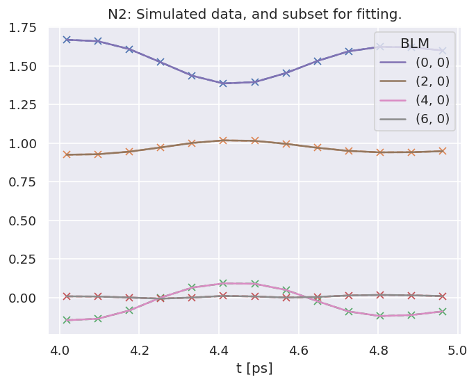
For radial matrix elements retrieval problems based on RWP methods, the absolute degree of alignment may - or may not - be critical in a given case. The sampling of a range of different alignments, however, is vital, since this directly feeds into the information content of the measurements (see Sect. 3.3.8 and Sect. 3.7). In the case-studies of Part II, the ADMs are assumed to be known, but in general these must be determined from experimental data, this is discussed in Sect. 4.1.1.

3.5.2. Alignment distribution moments (ADMs)#

The parametrization of an aligned distribution can be given generally by an expansion in Wigner rotation matrix elements:

(3.35)#\[ P(\Omega,t) = \sum_{K,Q,S} A^K_{Q,S}(t)D^K_{Q,S}(\Omega) \]

Where \(P(\Omega,t)\) is the full axis distribution probability, expanded for a set of Euler angles \(\Omega\), and the expansion parameters \(A^K_{Q,S}(t)\) are the ADMs.

This reduces to the 2D case if \(S=0\), which can equivalently be described as an expansion in spherical harmonics (note that the normalisation of the ADMs may be different in this case):

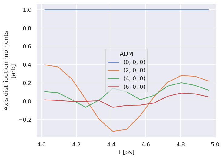
(3.36)#\[ P(\theta,\phi,t) = \sum_{K,Q} A^K_{Q,0}(t)D^K_{Q,0}(\Omega) = \sum_{K,Q} A^K_{Q}(t)Y_{K,Q}(\Omega) \]

In the examples given in Sect. 3.3, some arbitrary choices of \(A^K_{Q,S}(t)\) were demonstrated to investigate their effects on the tensor basis sets; in the case-studies presented in Part II realistic ADMs are used for specific fitting problems. In practice this equates to (accurately) simulating rotational wavepackets, hence obtaining the corresponding \(A_{Q,S}^{K}(t)\) parameters (expectation values), as a function of laser fluence and rotational temperature. (Given experimental data, a 2D uncertainty (or error) surface in these two fundamental quantities can then be obtained from a linear regression for each set of \(A_{Q,S}^{K}(t)\), see Ref. [3] for further introductory discussion on this point.) Note that, as discussed in Sect. 2.5, computation of molecular alignment is not yet implemented in the Photoelectron Metrology Toolkit [5], so values must be obtained from other codes. ADMs used herein were all computed with codes developed by V. Makhija [116], and are available from the ePSproc [34] repo on Github.

3.5.3. Numerical setup#

For illustrative purposes, the ADMs used for the \(N_2\) fitting example are here loaded and used to compute \(P(\Omega,t)\). (Note these ADMs are for a 2-pulse alignment scheme, as outlined in Ref. [1].)

Show code cell content Hide code cell content

# %matplotlib inline

# Pass custom img config for notebook
# import os
# os.environ['IMGWIDTH']='750'
# Run default config - may need to set full path here
# %run '../scripts/setup_notebook.py'
%run '../scripts/setup_notebook_caseStudies_Mod-300723.py'   # Test version with different figure options.

# Run OCS setup script - may need to set full path here
# ADMfile = 'ADMs_8TW_120fs_5K.mat'
# dataPath = Path('../part2/OCSfitting')
# dataPath = Path('/home/jovyan/QM3/doc-source/part2/OCSfitting')

# Run general config script with dataPath set above
# %run {dataPath/"setup_fit_demo_OCS.py"} -d {dataPath} -a {dataPath} -c "OCS"

# 29/07/23 - updated scripts
# For sample ADMs, set 'N2', 'OCS' or 'C2H4' - see case study chapters for details.
fitSystem='N2'
dataName = 'n2fitting'
dataPath = Path(Path.cwd().parent,'part2',dataName)

# Run general config script with dataPath set above
%run "../scripts/setup_fit_case-studies_270723.py" -d {dataPath} -c {fitSystem}

*** Setting up notebook with standard Quantum Metrology Vol. 3 imports...
For more details see https://pemtk.readthedocs.io/en/latest/fitting/PEMtk_fitting_basic_demo_030621-full.html
To use local source code, pass the parent path to this script at run time, e.g. "setup_fit_demo ~/github"

*** Running: 2023-12-07 10:44:07
Working dir: /home/jovyan/jake-home/buildTmp/_latest_build/html/doc-source/part1
Build env: html
None

* Loading packages...
* sparse not found, sparse matrix forms not available. 
* natsort not found, some sorting functions not available. 
* Setting plotter defaults with epsproc.basicPlotters.setPlotters(). Run directly to modify, or change options in local env.
* Set Holoviews with bokeh.
* pyevtk not found, VTK export not available. 
* Set Holoviews with bokeh.
Jupyter Book      : 0.15.1
External ToC      : 0.3.1
MyST-Parser       : 0.18.1
MyST-NB           : 0.17.2
Sphinx Book Theme : 1.0.1
Jupyter-Cache     : 0.6.1
NbClient          : 0.7.4
*** Setting up demo fitting workspace and main `data` class object...
Script: QM3 case studies
For more details see https://pemtk.readthedocs.io/en/latest/fitting/PEMtk_fitting_basic_demo_030621-full.html
To use local source code, pass the parent path to this script at run time, e.g. "setup_fit_demo ~/github"


* Loading packages...

* Loading demo matrix element data from /home/jovyan/jake-home/buildTmp/_latest_build/html/doc-source/part2/n2fitting

*** Job subset details
Key: subset
No 'job' info set for self.data[subset].

*** Job orb6 details
Key: orb6
Dir /home/jovyan/jake-home/buildTmp/_latest_build/html/doc-source/part2/n2fitting, 1 file(s).
{   'batch': 'ePS n2, batch n2_1pu_0.1-50.1eV, orbital A2',
    'event': ' N2 A-state (1piu-1)',
    'orbE': -17.09691397835426,
    'orbLabel': '1piu-1'}

*** Job orb5 details
Key: orb5
Dir /home/jovyan/jake-home/buildTmp/_latest_build/html/doc-source/part2/n2fitting, 1 file(s).
{   'batch': 'ePS n2, batch n2_3sg_0.1-50.1eV, orbital A2',
    'event': ' N2 X-state (3sg-1)',
    'orbE': -17.34181645456815,
    'orbLabel': '3sg-1'}

*** Job subset details
Key: subset
No 'job' info set for self.data[subset].

*** Job orb6 details
Key: orb6
Dir /home/jovyan/jake-home/buildTmp/_latest_build/html/doc-source/part2/n2fitting, 1 file(s).
{   'batch': 'ePS n2, batch n2_1pu_0.1-50.1eV, orbital A2',
    'event': ' N2 A-state (1piu-1)',
    'orbE': -17.09691397835426,
    'orbLabel': '1piu-1'}

*** Job orb5 details
Key: orb5
Dir /home/jovyan/jake-home/buildTmp/_latest_build/html/doc-source/part2/n2fitting, 1 file(s).
{   'batch': 'ePS n2, batch n2_3sg_0.1-50.1eV, orbital A2',
    'event': ' N2 X-state (3sg-1)',
    'orbE': -17.34181645456815,
    'orbLabel': '3sg-1'}
*** Running with default N2 settings.


* Loading demo ADM data from file /home/jovyan/jake-home/buildTmp/_latest_build/html/doc-source/part2/n2fitting/N2_ADM_VM_290816.mat...

* Subselecting data...
*** Setting for N2 case study.
Subselected from dataset 'orb5', dataType 'matE': 36 from 11016 points (0.33%)
Subselected from dataset 'pol', dataType 'pol': 1 from 3 points (33.33%)
Subselected from dataset 'ADM', dataType 'ADM': 52 from 14764 points (0.35%)

* Calculating AF-BLMs...

Running for 13 t-points
Subselected from dataset 'sim', dataType 'AFBLM': 52 from 52 points (100.00%)

*Setting  up fit parameters (with constraints)...
Set 6 complex matrix elements to 12 fitting params, see self.params for details.
Auto-setting parameters.
Basis set size = 12 params. Fitting with 4 magnitudes and 3 phases floated.


*** Setup demo fitting workspace OK.
Dataset: subset, AFBLM
Dataset: sim, AFBLM

Parameters
name	value	initial value	min	max	vary	expression
m_PU_SG_PU_1_n1_1_1	1.78461575	1.784615753610107	1.0000e-04	5.00000000	True
m_PU_SG_PU_1_1_n1_1	1.78461575	1.784615753610107	1.0000e-04	5.00000000	False	m_PU_SG_PU_1_n1_1_1
m_PU_SG_PU_3_n1_1_1	0.80290495	0.802904951323892	1.0000e-04	5.00000000	True
m_PU_SG_PU_3_1_n1_1	0.80290495	0.802904951323892	1.0000e-04	5.00000000	False	m_PU_SG_PU_3_n1_1_1
m_SU_SG_SU_1_0_0_1	2.68606212	2.686062120382649	1.0000e-04	5.00000000	True
m_SU_SG_SU_3_0_0_1	1.10915311	1.109153108617096	1.0000e-04	5.00000000	True
p_PU_SG_PU_1_n1_1_1	-0.86104140	-0.8610414024232179	-3.14159265	3.14159265	False
p_PU_SG_PU_1_1_n1_1	-0.86104140	-0.8610414024232179	-3.14159265	3.14159265	False	p_PU_SG_PU_1_n1_1_1
p_PU_SG_PU_3_n1_1_1	-3.12044446	-3.1204444620772467	-3.14159265	3.14159265	True
p_PU_SG_PU_3_1_n1_1	-3.12044446	-3.1204444620772467	-3.14159265	3.14159265	False	p_PU_SG_PU_3_n1_1_1
p_SU_SG_SU_1_0_0_1	2.61122920	2.611229196458127	-3.14159265	3.14159265	True
p_SU_SG_SU_3_0_0_1	-0.07867828	-0.07867827542158025	-3.14159265	3.14159265	True

../_images/50580861a07ad92f5b8765b6ec4f5430a0820088c10995510c088ec1ddc886b5.png

# Quick plot for subselected ADMs (setup in the script), 
# using basic plotter
data.ADMplot(keys = data.subKey)

# Quick plot for subselected ADMs (setup in the script), using hvplot
# data.data['subset']['ADM'].unstack().squeeze().real.hvplot.line(x='t').overlay('K')

# As above, but plot K>0 terms only, and keep 'Q','S' indexes (here all =0)
figObj = data.data['subset']['ADM'].unstack().where(data.data['subset']['ADM'].unstack().K>0) \
        .real.hvplot.line(x='t').overlay(['K','Q','S']).opts(width=700)

# Glue plot for later
glue("fitSystem", fitSystem, display=False)
glue("ADMdemoPlot", figObj)

Fig. 3.14 Example ADMs for N2.#

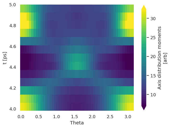
3.5.4. Compute \(P(\theta,\Phi,t)\) distributions#

For 1D and 2D cases, the full axis distributions can be expanded in spherical harmonics and plotted using Photoelectron Metrology Toolkit [5] class methods. This is briefly illustrated below. Note that expansions in Wigner rotation matrix elements are not currently supported by these routines.

# NOTE - need this in some builds if Matplotlib has call-back errors.
%matplotlib inline  
# Plot P(theta,t) with summation over phi dimension
# Note the plotting function automatically expands the ADMs in spherical harmonics
dataKey = 'subset'
data.padPlot(keys = dataKey, dataType='ADM', Etype = 't', pStyle='grid', reducePhi='sum', returnFlag = True)

Using default sph betas.
Summing over dims: set()
Plotting from self.data[subset][ADM], facetDims=['t', None], pType=a with backend=mpl.
Grid plot: ('subset', 'ADM'), dataType: ADM, plotType: a
Set plot to self.data['subset']['plots']['ADM']['grid']

../_images/552a5788e8ea3eb18ca2105b2d8355a293903da7102e66dcfcd0caf027301e47.png

# Plot full axis distributions at selected time-steps
# tPlot = [39.402, 40.791, 42.18]  # Manual setting for baseline case, and at max and min K=2 times. OCS
tPlot = [4.018, 4.254, 4.49] # N2

# Alternatively, plot at selected times by index slice
# Note that selDims below requires labels (not index inds)
# tPlot = data.data[dataKey]['ADM'].t[::5]  # OCS
# tPlot = data.data[dataKey]['ADM'].t[0:7:3] # N2

# Plot
ep.plot.hvPlotters.setPlotters(width=1200, height=600)   # Force plot dims for HTML render (avoids subplot clipping issues)
data.padPlot(keys = dataKey, dataType='ADM', Etype = 't', pType='a', 
             returnFlag = True, selDims={'t':tPlot}, backend='pl')

# And GLUE for display later with caption
figObj = data.data[dataKey]['plots']['ADM']['polar'][0]
glue("axisDistDemo", figObj)

Fig. 3.15 Molecular axis distributions \(P(\theta,\phi)\) at selected times. In this demo case the alignment is “1D”, and cylindrically symmetric.#