7. General fit setup and numerics#
For the case studies in Chapter 8 - 10, the same basic setup and fitting routine is used in all cases, and this is outlined below. In general, this requires the steps outlined in Chpt. 6 and, for the case studies, configuration additionally requires ePolyScat (ePS) [36, 37, 38, 39] ab initio radial matrix elements, and ADMs, in order to define test datasets (Sect. 7.3). The \(N_2\) case study is use as an example in this case, and Sect. 7.4 illustrates both setting test data, and running fits. Additionally, for the case studies herein, the setup routines are wrapped in a basic script, with configuration options for each case included, this is illustrated in Sect. 7.4.4.
For the case studies, all the sample data is available from the ePSproc [34] Github repo, and the examples below include steps for pulling the required data files. Note that further ePolyScat (ePS) [36, 37, 38, 39] datasets are available from ePSdata [48], and data can be pulled using the python ePSdata interface.
7.1. Init and pulling data#
Here the setup is mainly handled by some basic scripts, these follow the outline in the PEMtk documentation [20], see in particular the intro to fitting.
Show code cell content
# Run default config - may need to set full path here
%run '../scripts/setup_notebook.py'

# Override plotters backend?
# plotBackend = 'pl'
*** Setting up notebook with standard Quantum Metrology Vol. 3 imports...
For more details see https://pemtk.readthedocs.io/en/latest/fitting/PEMtk_fitting_basic_demo_030621-full.html
To use local source code, pass the parent path to this script at run time, e.g. "setup_fit_demo ~/github"

*** Running: 2023-12-07 10:45:25
Working dir: /home/jovyan/jake-home/buildTmp/_latest_build/html/doc-source/part2
Build env: html
None

* Loading packages...
* sparse not found, sparse matrix forms not available.
* natsort not found, some sorting functions not available.
* Setting plotter defaults with epsproc.basicPlotters.setPlotters(). Run directly to modify, or change options in local env.
* Set Holoviews with bokeh.
* pyevtk not found, VTK export not available.
* Set Holoviews with bokeh.
Jupyter Book      : 0.15.1
External ToC      : 0.3.1
MyST-Parser       : 0.18.1
MyST-NB           : 0.17.2
Sphinx Book Theme : 1.0.1
Jupyter-Cache     : 0.6.1
NbClient          : 0.7.4
# Pull data files as required from Github, note the path here is required

# *** Method using epsproc.util.io.getFilesFromGithub
# For pulling data from Github, a utility function is available
# This requires the repo subpath, and optionally branch
# The function will pull all files found in the repo path
from epsproc.util.io import getFilesFromGithub

# Set dataName (will be used as download subdir)
dataName = 'n2fitting'
# N2 matrix elements
fDictMatE, fAllMatE = getFilesFromGithub(subpath='data/photoionization/n2_multiorb', dataName=dataName)
# N2 alignment data
fDictADM, fAllMatADM = getFilesFromGithub(subpath='data/alignment', dataName=dataName)

# *** Alternative method: supply URLs directly for file downloader
# E.g. Pull N2 data from ePSproc Github repo

# URLs for test ePSproc datasets - n2
# For more datasets use ePSdata, see https://epsproc.readthedocs.io/en/dev/demos/ePSdata_download_demo_300720.html
urls = {'n2PU':"https://github.com/phockett/ePSproc/blob/master/data/photoionization/n2_multiorb/n2_1pu_0.1-50.1eV_A2.inp.out",
        'n2SU':"https://github.com/phockett/ePSproc/blob/master/data/photoionization/n2_multiorb/n2_3sg_0.1-50.1eV_A2.inp.out",
        'n2ADMs':"https://github.com/phockett/ePSproc/blob/master/data/alignment/N2_ADM_VM_290816.mat",
        'demoScript':"https://github.com/phockett/PEMtk/blob/master/demos/fitting/setup_fit_demo.py"}

from epsproc.util.io import getFilesFromURLs
fList, fDict = getFilesFromURLs(urls, dataName=dataName)
Querying URL: https://api.github.com/repos/phockett/epsproc/contents/data/photoionization/n2_multiorb
Local file /home/jovyan/jake-home/buildTmp/_latest_build/html/doc-source/part2/n2fitting/n2_1pu_0.1-50.1eV_A2.inp.out already exists
Local file /home/jovyan/jake-home/buildTmp/_latest_build/html/doc-source/part2/n2fitting/n2_3sg_0.1-50.1eV_A2.inp.out already exists
Querying URL: https://api.github.com/repos/phockett/epsproc/contents/data/alignment
Local file /home/jovyan/jake-home/buildTmp/_latest_build/html/doc-source/part2/n2fitting/N2_ADM_VM_290816.mat already exists
Local file /home/jovyan/jake-home/buildTmp/_latest_build/html/doc-source/part2/n2fitting/n2_1pu_0.1-50.1eV_A2.inp.out already exists
Local file /home/jovyan/jake-home/buildTmp/_latest_build/html/doc-source/part2/n2fitting/n2_3sg_0.1-50.1eV_A2.inp.out already exists
Local file /home/jovyan/jake-home/buildTmp/_latest_build/html/doc-source/part2/n2fitting/N2_ADM_VM_290816.mat already exists
Downloading from https://github.com/phockett/PEMtk/blob/master/demos/fitting/setup_fit_demo.py to /home/jovyan/jake-home/buildTmp/_latest_build/html/doc-source/part2/n2fitting/setup_fit_demo.py.
Pulled to file: /home/jovyan/jake-home/buildTmp/_latest_build/html/doc-source/part2/n2fitting/setup_fit_demo.py
7.2. Setup with options#
Following the PEMtk documentation [20], the fitting workspace can be configured by setting:
A fitting basis set, either from computational matrix elements, from symmetry constraints, or manually. (See Chpt. 6 for more discussion.)
Data to fit. In the examples herein synthetic data will be created by adding noise to computational results.
ADMs to use for the fit. Again these may be from computational results, or set manually. If not specified these will default to an isotropic distribution, which may be appropriate in some cases.
In the following subsections each aspect of the configuration is illustrated.
# Initiation - a PEMtk fitting class object

# Set data dir
dataPath = Path(Path.cwd(), dataName)

# Init class object
data = pemtkFit(fileBase = dataPath, verbose = 1)

# Read data files
data.scanFiles()
*** Job subset details
Key: subset
No 'job' info set for self.data[subset].

*** Job orb6 details
Key: orb6
Dir /home/jovyan/jake-home/buildTmp/_latest_build/html/doc-source/part2/n2fitting, 1 file(s).
{   'batch': 'ePS n2, batch n2_1pu_0.1-50.1eV, orbital A2',
    'event': ' N2 A-state (1piu-1)',
    'orbE': -17.09691397835426,
    'orbLabel': '1piu-1'}

*** Job orb5 details
Key: orb5
Dir /home/jovyan/jake-home/buildTmp/_latest_build/html/doc-source/part2/n2fitting, 1 file(s).
{   'batch': 'ePS n2, batch n2_3sg_0.1-50.1eV, orbital A2',
    'event': ' N2 X-state (3sg-1)',
    'orbE': -17.34181645456815,
    'orbLabel': '3sg-1'}
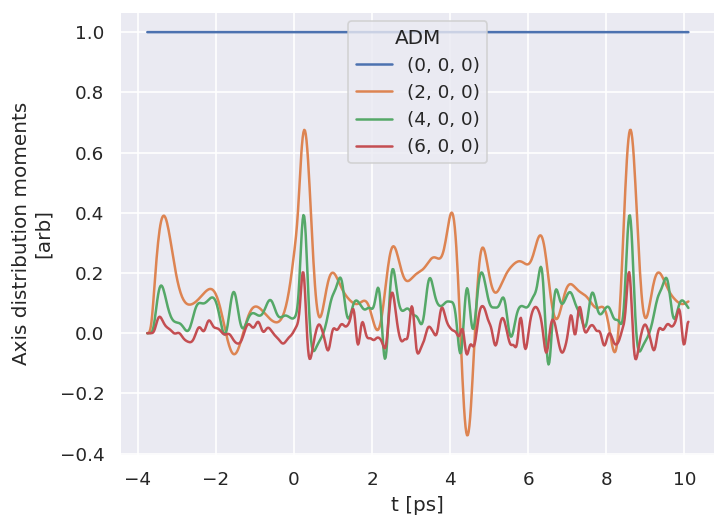
7.2.1. Alignment distribution moments (ADMs)#
The class wraps ep.setADMs() to set ADMs to the class data structure. This returns an isotropic distribution by default, or values can be set explicitly from a list. Note: if this is not set, the default value will be used, which is likely not very useful for the fit!
Values are set in self.data['ADM'], see Sect. 3.5 for more details on ADMs and molecular alignment. For the \(N_2\) example case, the alignment data is as per the original experimental demonstration of the bootstrap retrieval protocol [1], and also available from the associated data repository [143].
# Default case - isotropic
data.setADMs()
# data.ADM['ADMX']
data.data['ADM']['ADM']
<xarray.DataArray 'ADM' (ADM: 1, t: 1)>
array([[1]])
Coordinates:
  * ADM      (ADM) MultiIndex
  - K        (ADM) int64 0
  - Q        (ADM) int64 0
  - S        (ADM) int64 0
  * t        (t) int64 0
Attributes:
    dataType:   ADM
    long_name:  Axis distribution moments
units: arb# Load time-dependent ADMs for N2 case
# These are in a Matlab/HDF5 file format
from scipy.io import loadmat
ADMdataFile = os.path.join(dataPath, 'N2_ADM_VM_290816.mat')
ADMs = loadmat(ADMdataFile)
# Set tOffset for calcs, 3.76ps!!!
# This is because this is 2-pulse case, and will set t=0 to 2nd pulse
# (and matches defn. in N2 experimental paper)
# Marceau, C. et al. (2017) ‘Molecular Frame Reconstruction Using Time-Domain Photoionization Interferometry’, Physical Review Letters, 119(8), p. 083401. Available at: https://doi.org/10.1103/PhysRevLett.119.083401.
tOffset = -3.76
ADMs['time'] = ADMs['time'] + tOffset
data.setADMs(ADMs = ADMs['ADM'], t=ADMs['time'].squeeze(), KQSLabels = ADMs['ADMlist'], addS = True)
data.data['ADM']['ADM']
<xarray.DataArray 'ADM' (ADM: 4, t: 3691)>
array([[ 1.00000000e+00+0.00000000e+00j,  1.00000000e+00+0.00000000e+00j,
         1.00000000e+00+0.00000000e+00j, ...,
         1.00000000e+00+0.00000000e+00j,  1.00000000e+00+0.00000000e+00j,
         1.00000000e+00+0.00000000e+00j],
       [-2.26243113e-17+0.00000000e+00j,  2.43430608e-08+1.04125246e-20j,
         9.80188266e-08+6.89166168e-20j, ...,
         1.05433798e-01-1.62495135e-18j,  1.05433798e-01-1.62495135e-18j,
         1.05433798e-01-1.62495135e-18j],
       [ 1.55724057e-16+0.00000000e+00j, -3.37021111e-10-6.81416260e-20j,
         1.95424253e-10-3.10513374e-19j, ...,
         8.39913132e-02-5.12795441e-17j,  8.39913132e-02-5.12795441e-17j,
         8.39913132e-02-5.12795441e-17j],
       [-7.68430227e-16+0.00000000e+00j, -1.40177466e-11+1.04987400e-19j,
         6.33419102e-10+1.74747003e-18j, ...,
         3.78131657e-02+4.01318983e-16j,  3.78131657e-02+4.01318983e-16j,
         3.78131657e-02+4.01318983e-16j]])
Coordinates:
  * ADM      (ADM) MultiIndex
  - K        (ADM) int64 0 2 4 6
  - Q        (ADM) int64 0 0 0 0
  - S        (ADM) int64 0 0 0 0
  * t        (t) float64 -3.76 -3.76 -3.76 -3.759 -3.759 ... 10.1 10.1 10.1 10.1
Attributes:
    dataType:   ADM
    long_name:  Axis distribution moments
units: arb# Manual plot with hvplot for full control and interactive plot
# NOTE: HTML version only.
key = 'ADM'
dataType='ADM'
data.data[key][dataType].unstack().real.hvplot.line(x='t').overlay(['K','Q','S'])
# A basic self.ADMplot routine is also available
%matplotlib inline
data.ADMplot(keys = 'ADM')
Dataset: ADM, ADM
7.2.2. Polarisation geometry/ies#
This wraps ep.setPolGeoms. This defaults to (x,y,z) polarization geometries. Values are set in self.data['pol'].
Note: if this is not set, the default value will be used, which is likely not very useful for the fit!
data.setPolGeoms()
data.data['pol']['pol']
<xarray.DataArray (Labels: 3)>
array([quaternion(1, -0, 0, 0),
       quaternion(0.707106781186548, -0, 0.707106781186547, 0),
       quaternion(0.5, -0.5, 0.5, 0.5)], dtype=quaternion)
Coordinates:
    Euler    (Labels) object (0.0, 0.0, 0.0) ... (1.5707963267948966, 1.57079...
  * Labels   (Labels) <U32 'z' 'x' 'y'
Attributes:
dataType: Euler7.2.3. Subselect data#
Currently handled in the class by setting self.selOpts, this allows for simple reuse of settings as required. Subselected data is set to self.data['subset'][dataType] by default (equivalently self.data[self.subKey][dataType]), and is the data the fitting routine will use.
# Settings for type subselection are in selOpts[dataType]
# E.g. Matrix element sub-selection
data.selOpts['matE'] = {'thres': 0.01, 'inds': {'Type':'L', 'Eke':1.1}}
data.setSubset(dataKey = 'orb5', dataType = 'matE') # Subselect from 'orb5' dataset, matrix elements
# And for the polarisation geometries...
data.selOpts['pol'] = {'inds': {'Labels': 'z'}}
data.setSubset(dataKey = 'pol', dataType = 'pol')
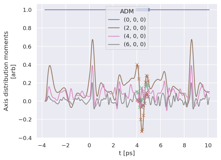
# And for the ADMs...
data.selOpts['ADM'] = {} #{'thres': 0.01, 'inds': {'Type':'L', 'Eke':1.1}}
data.setSubset(dataKey = 'ADM', dataType = 'ADM', sliceParams = {'t':[4, 5, 4]})
Subselected from dataset 'orb5', dataType 'matE': 36 from 11016 points (0.33%)
Subselected from dataset 'pol', dataType 'pol': 1 from 3 points (33.33%)
Subselected from dataset 'ADM', dataType 'ADM': 52 from 14764 points (0.35%)
# Note that the class uses data.subKey to reference the correct data internally
print(f'Data dict key: {data.subKey}')
print(f'Data dict contents: {data.data[data.subKey].keys()}')
Data dict key: subset
Data dict contents: dict_keys(['matE', 'pol', 'ADM'])
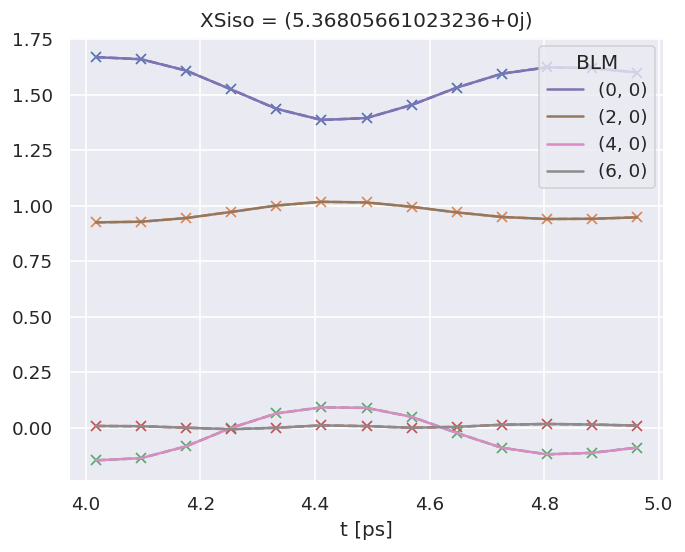
# Check subselected ADMs by plotting vs. full ADM data
# Plot from Xarray vs. full dataset
data.data['subset']['ADM'].real.squeeze().plot.line(x='t', marker = 'x', linestyle='dashed');
data.data['ADM']['ADM'].real.squeeze().plot.line(x='t');
7.3. Compute AF-\(\beta_{LM}\) and simulate data#
With all the components set, some observables can be calculated. For testing, this will also be used to simulate an experimental trace (with noise added).
For both basic computation, and fitting, the class method self.afblmMatEfit() can be used. This essentially wraps the main AF computational routine, epsproc.afblmXprod(), to compute AF-\(\beta_{LM}\)s (for more details, see the ePSproc method development docs and API docs).
If called without reference data, the method returns computed AF-\(\beta_{LM}\)s based on the input subsets already created, and also a set of (product) basis functions generated - as illustrated in Sect. 3.3, these can be examined to get a feel for the sensitivity of the geometric part of the problem, and will also be used as a basis in the fitting routine to limit repetitive computations.
7.3.1. Compute AF-\(\beta_{LM}\)s#
# Compute with class method
# This uses all data as set to self.data['subset']
BetaNormX, basis = data.afblmMatEfit()
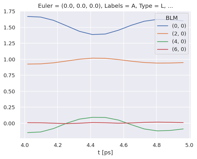
7.3.2. AF-\(\beta_{LM}\)s#
The returned objects contain the \(\beta_{LM}\) parameters as an Xarray…
# Line-plot with Xarray/Matplotlib
# Note there is no filtering here, so this includes some invalid and null terms
BetaNormX.sel(Labels='A').real.squeeze().plot.line(x='t');
… and the basis sets as a dictionary. (See Sect. 3.3 for more details on the basis sets.)
basis.keys()
dict_keys(['BLMtableResort', 'polProd', 'phaseConvention', 'BLMRenorm'])
7.4. Fitting the data: configuration#
As discussed in Chpt. 4, general non-linear fitting approaches are used for the bootstrap retrieval protocol. These are wrapped in the Photoelectron Metrology Toolkit [5] for radial matrix elements retrieval problems, as shown below. (And, as discussed in Sect. 2.3, make use of the lmfit library [66, 67] and Scipy [52] base routines.)
7.4.1. Set the data to fit#
To use the values calculated above as the test data, it currently needs to be set as self.data['subset']['AFBLM'] for fitting.
# Set computed results to main data structure

# Method 1: Set directly by manual assignment
# data.data['subset']['AFBLM'] = BetaNormX

# Method 2: Set to main data structure and subset using methods as above
# Set simulated data to master structure as "sim"
data.setData('sim', BetaNormX)
# Set to 'subset' to use for fitting.
data.setSubset('sim','AFBLM')
Subselected from dataset 'sim', dataType 'AFBLM': 52 from 52 points (100.00%)
# Set basis functions
data.basis = basis
7.4.2. Adding noise#
For a more realistic test of the bootstrap retrieval protocol, noise or other artifacts can be added to the data. Below is a routine for adding random (Gaussian) noise.
# Add noise with np.random.normal
# https://numpy.org/doc/stable/reference/random/generated/numpy.random.normal.html
import numpy as np
mu, sigma = 0, 0.05 # Up to approx 10% noise (+/- 0.05)
# creating a noise with the same dimension as the dataset (2,2)
noise = np.random.normal(mu, sigma,
[data.data['subset']['AFBLM'].t.size,
data.data['subset']['AFBLM'].l.size])
# data.BLMfitPlot()
# Set noise in Xarray & scale by l
import xarray as xr
noiseXR = xr.ones_like(data.data['subset']['AFBLM']) * noise
# Scale by L? This prevents too much high-order noise
noiseXR = noiseXR.where(noiseXR.l<1, noiseXR/(noiseXR.l))
# Update data for fitting
data.data['subset']['AFBLM'] = data.data['subset']['AFBLM'] + noiseXR
# Remove non-zero m terms?
# This removes additional noise-only channels
data.data['subset']['AFBLM'] = data.data['subset']['AFBLM'].where(data.data['subset']['AFBLM'].m == 0, 0)
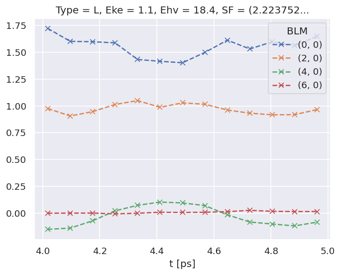
# The BLMfitPlot() routine can be used to plot data and fit outputs
data.BLMfitPlot()
Dataset: subset, AFBLM
7.4.3. Setting up the fit parameters#
As detailed in Chpt. 6, fitting requires a basis set and fit parameters. In this case, we can work from the existing matrix elements (as used for simulating data above) to speed up parameter creation, although in practice this may need to be approached ab initio or via symmetry - nonetheless, the method will be similar.
# Set matrix elements from ab initio results
data.setMatEFit(data.data['subset']['matE'])
Show code cell output
Set 6 complex matrix elements to 12 fitting params, see self.params for details.
Auto-setting parameters.
| name | value | initial value | min | max | vary | expression |
|---|---|---|---|---|---|---|
| m_PU_SG_PU_1_n1_1_1 | 1.78461575 | 1.784615753610107 | 1.0000e-04 | 5.00000000 | True | |
| m_PU_SG_PU_1_1_n1_1 | 1.78461575 | 1.784615753610107 | 1.0000e-04 | 5.00000000 | False | m_PU_SG_PU_1_n1_1_1 |
| m_PU_SG_PU_3_n1_1_1 | 0.80290495 | 0.802904951323892 | 1.0000e-04 | 5.00000000 | True | |
| m_PU_SG_PU_3_1_n1_1 | 0.80290495 | 0.802904951323892 | 1.0000e-04 | 5.00000000 | False | m_PU_SG_PU_3_n1_1_1 |
| m_SU_SG_SU_1_0_0_1 | 2.68606212 | 2.686062120382649 | 1.0000e-04 | 5.00000000 | True | |
| m_SU_SG_SU_3_0_0_1 | 1.10915311 | 1.109153108617096 | 1.0000e-04 | 5.00000000 | True | |
| p_PU_SG_PU_1_n1_1_1 | -0.86104140 | -0.8610414024232179 | -3.14159265 | 3.14159265 | False | |
| p_PU_SG_PU_1_1_n1_1 | -0.86104140 | -0.8610414024232179 | -3.14159265 | 3.14159265 | False | p_PU_SG_PU_1_n1_1_1 |
| p_PU_SG_PU_3_n1_1_1 | -3.12044446 | -3.1204444620772467 | -3.14159265 | 3.14159265 | True | |
| p_PU_SG_PU_3_1_n1_1 | -3.12044446 | -3.1204444620772467 | -3.14159265 | 3.14159265 | False | p_PU_SG_PU_3_n1_1_1 |
| p_SU_SG_SU_1_0_0_1 | 2.61122920 | 2.611229196458127 | -3.14159265 | 3.14159265 | True | |
| p_SU_SG_SU_3_0_0_1 | -0.07867828 | -0.07867827542158025 | -3.14159265 | 3.14159265 | True |
This sets self.params from the matrix elements, which are a set of (real) parameters for lmfit, as a Parameters object.
Note that:
The input matrix elements are converted to magnitude-phase form, hence there are twice the number as the input array, and labelled
morpaccordingly, along with a name based on the full set of QNs/indexes set.One phase is set to
vary=False, which defines a reference phase. This defaults to the first phase item.Min and max values are defined, by default the ranges are \(1e^{-4}<\)mag\(<5\), \(-\pi<\)phase\(<\pi\).
Relationships between the parameters are set by default, but can be set manually, or pass
paramsCons=Noneto skip.
For further details, including modification of parameter settings, see Sect. 6.3.4.2 and the PEMtk documentation [20].
7.4.4. Quick setup with script#
The steps demonstrated above are also wrapped in a helper script, although some steps may need to be re-run to change selection properties or ranges. For the case studies, there are specific details for each configured in the script, including source data locations and the selection criteria as used in each demonstration.
# Run general config script with dataPath set above
%run {dataPath/"setup_fit_demo.py"} -d {dataPath}
Show code cell output
*** Setting up demo fitting workspace and main `data` class object...
For more details see https://pemtk.readthedocs.io/en/latest/fitting/PEMtk_fitting_basic_demo_030621-full.html
To use local source code, pass the parent path to this script at run time, e.g. "setup_fit_demo ~/github"


* Loading packages...
* Set Holoviews with bokeh.

* Loading demo matrix element data from /home/jovyan/jake-home/buildTmp/_latest_build/html/doc-source/part2/n2fitting

*** Job subset details
Key: subset
No 'job' info set for self.data[subset].

*** Job orb6 details
Key: orb6
Dir /home/jovyan/jake-home/buildTmp/_latest_build/html/doc-source/part2/n2fitting, 1 file(s).
{   'batch': 'ePS n2, batch n2_1pu_0.1-50.1eV, orbital A2',
    'event': ' N2 A-state (1piu-1)',
    'orbE': -17.09691397835426,
    'orbLabel': '1piu-1'}

*** Job orb5 details
Key: orb5
Dir /home/jovyan/jake-home/buildTmp/_latest_build/html/doc-source/part2/n2fitting, 1 file(s).
{   'batch': 'ePS n2, batch n2_3sg_0.1-50.1eV, orbital A2',
    'event': ' N2 X-state (3sg-1)',
    'orbE': -17.34181645456815,
    'orbLabel': '3sg-1'}


* Loading demo ADM data from /home/jovyan/jake-home/buildTmp/_latest_build/html/doc-source/part2/n2fitting/N2_ADM_VM_290816.mat...

* Subselecting data...
Subselected from dataset 'orb5', dataType 'matE': 36 from 11016 points (0.33%)
Subselected from dataset 'pol', dataType 'pol': 1 from 3 points (33.33%)
Subselected from dataset 'ADM', dataType 'ADM': 52 from 14764 points (0.35%)

* Calculating AF-BLMs...
Subselected from dataset 'sim', dataType 'AFBLM': 52 from 52 points (100.00%)

*Setting  up fit parameters (with constraints)...
Set 6 complex matrix elements to 12 fitting params, see self.params for details.
Auto-setting parameters.


*** Setup demo fitting workspace OK.


| name | value | initial value | min | max | vary | expression |
|---|---|---|---|---|---|---|
| m_PU_SG_PU_1_n1_1_1 | 1.78461575 | 1.784615753610107 | 1.0000e-04 | 5.00000000 | True | |
| m_PU_SG_PU_1_1_n1_1 | 1.78461575 | 1.784615753610107 | 1.0000e-04 | 5.00000000 | False | m_PU_SG_PU_1_n1_1_1 |
| m_PU_SG_PU_3_n1_1_1 | 0.80290495 | 0.802904951323892 | 1.0000e-04 | 5.00000000 | True | |
| m_PU_SG_PU_3_1_n1_1 | 0.80290495 | 0.802904951323892 | 1.0000e-04 | 5.00000000 | False | m_PU_SG_PU_3_n1_1_1 |
| m_SU_SG_SU_1_0_0_1 | 2.68606212 | 2.686062120382649 | 1.0000e-04 | 5.00000000 | True | |
| m_SU_SG_SU_3_0_0_1 | 1.10915311 | 1.109153108617096 | 1.0000e-04 | 5.00000000 | True | |
| p_PU_SG_PU_1_n1_1_1 | -0.86104140 | -0.8610414024232179 | -3.14159265 | 3.14159265 | False | |
| p_PU_SG_PU_1_1_n1_1 | -0.86104140 | -0.8610414024232179 | -3.14159265 | 3.14159265 | False | p_PU_SG_PU_1_n1_1_1 |
| p_PU_SG_PU_3_n1_1_1 | -3.12044446 | -3.1204444620772467 | -3.14159265 | 3.14159265 | True | |
| p_PU_SG_PU_3_1_n1_1 | -3.12044446 | -3.1204444620772467 | -3.14159265 | 3.14159265 | False | p_PU_SG_PU_3_n1_1_1 |
| p_SU_SG_SU_1_0_0_1 | 2.61122920 | 2.611229196458127 | -3.14159265 | 3.14159265 | True | |
| p_SU_SG_SU_3_0_0_1 | -0.07867828 | -0.07867827542158025 | -3.14159265 | 3.14159265 | True |
<Figure size 768x576 with 0 Axes>
7.5. Fitting the data: Running fits#
7.5.1. Single fit#
With the parameters and data set, just call self.fit()! For more control, options to the lmfit library [66, 67] minimizer function can be set. Statistics and outputs are also handled by the lmfit library [66, 67], which includes uncertainty estimates and correlations in the fitted parameters.
# Run a fit
# data.randomizeParams()  # Randomize input parameters if desired
                          # For method testing using known initial params is also useful

# Run fit with defaults settings
data.fit()

# Additional keyword options can be pass, these are passed to the fitting routine.
# Args are passed to the lmfit minimizer, see https://lmfit.github.io/lmfit-py/fitting.html
# E.g. for scipy Least Squares, options can be found at
# https://docs.scipy.org/doc/scipy/reference/generated/scipy.optimize.least_squares.html#scipy.optimize.least_squares
# For example, pass convergence tolerances
# data.fit(ftol=1e-10, xtol=1e-10)
# Check fit outputs - self.result shows results from the last fit
data.result
Show code cell output
Fit Result
| fitting method | leastsq |
| # function evals | 9 |
| # data points | 52 |
| # variables | 7 |
| chi-square | 8.5896e-31 |
| reduced chi-square | 1.9088e-32 |
| Akaike info crit. | -3791.40336 |
| Bayesian info crit. | -3777.74466 |
| name | value | standard error | relative error | initial value | min | max | vary | expression |
|---|---|---|---|---|---|---|---|---|
| m_PU_SG_PU_1_n1_1_1 | 1.78461575 | 2.3594e-16 | (0.00%) | 1.784615753610107 | 1.0000e-04 | 5.00000000 | True | |
| m_PU_SG_PU_1_1_n1_1 | 1.78461575 | 2.3594e-16 | (0.00%) | 1.784615753610107 | 1.0000e-04 | 5.00000000 | False | m_PU_SG_PU_1_n1_1_1 |
| m_PU_SG_PU_3_n1_1_1 | 0.80290495 | 6.7716e-16 | (0.00%) | 0.802904951323892 | 1.0000e-04 | 5.00000000 | True | |
| m_PU_SG_PU_3_1_n1_1 | 0.80290495 | 6.7716e-16 | (0.00%) | 0.802904951323892 | 1.0000e-04 | 5.00000000 | False | m_PU_SG_PU_3_n1_1_1 |
| m_SU_SG_SU_1_0_0_1 | 2.68606212 | 1.3974e-15 | (0.00%) | 2.686062120382649 | 1.0000e-04 | 5.00000000 | True | |
| m_SU_SG_SU_3_0_0_1 | 1.10915311 | 3.3874e-15 | (0.00%) | 1.109153108617096 | 1.0000e-04 | 5.00000000 | True | |
| p_PU_SG_PU_1_n1_1_1 | -0.86104140 | 0.00000000 | (0.00%) | -0.8610414024232179 | -3.14159265 | 3.14159265 | False | |
| p_PU_SG_PU_1_1_n1_1 | -0.86104140 | 0.00000000 | (0.00%) | -0.8610414024232179 | -3.14159265 | 3.14159265 | False | p_PU_SG_PU_1_n1_1_1 |
| p_PU_SG_PU_3_n1_1_1 | -3.12044446 | 1.2883e-15 | (0.00%) | -3.1204444620772467 | -3.14159265 | 3.14159265 | True | |
| p_PU_SG_PU_3_1_n1_1 | -3.12044446 | 1.2883e-15 | (0.00%) | -3.1204444620772467 | -3.14159265 | 3.14159265 | False | p_PU_SG_PU_3_n1_1_1 |
| p_SU_SG_SU_1_0_0_1 | 2.61122920 | 9.0326e-16 | (0.00%) | 2.611229196458127 | -3.14159265 | 3.14159265 | True | |
| p_SU_SG_SU_3_0_0_1 | -0.07867828 | 3.7987e-15 | (0.00%) | -0.07867827542158025 | -3.14159265 | 3.14159265 | True |
| Parameter1 | Parameter 2 | Correlation |
|---|---|---|
| m_SU_SG_SU_1_0_0_1 | m_SU_SG_SU_3_0_0_1 | -0.9874 |
| p_SU_SG_SU_1_0_0_1 | p_SU_SG_SU_3_0_0_1 | -0.9098 |
| m_SU_SG_SU_3_0_0_1 | p_SU_SG_SU_3_0_0_1 | -0.8968 |
| m_SU_SG_SU_1_0_0_1 | p_SU_SG_SU_3_0_0_1 | +0.8855 |
| m_SU_SG_SU_1_0_0_1 | p_SU_SG_SU_1_0_0_1 | -0.8394 |
| m_SU_SG_SU_3_0_0_1 | p_SU_SG_SU_1_0_0_1 | +0.8261 |
| m_PU_SG_PU_1_n1_1_1 | m_PU_SG_PU_3_n1_1_1 | -0.7856 |
| m_PU_SG_PU_1_n1_1_1 | p_SU_SG_SU_1_0_0_1 | -0.5380 |
| m_PU_SG_PU_3_n1_1_1 | p_SU_SG_SU_1_0_0_1 | +0.4552 |
| p_PU_SG_PU_3_n1_1_1 | p_SU_SG_SU_3_0_0_1 | -0.3845 |
| m_PU_SG_PU_1_n1_1_1 | p_SU_SG_SU_3_0_0_1 | +0.2973 |
| m_PU_SG_PU_3_n1_1_1 | p_SU_SG_SU_3_0_0_1 | -0.1802 |
| m_SU_SG_SU_3_0_0_1 | p_PU_SG_PU_3_n1_1_1 | +0.1514 |
| m_PU_SG_PU_1_n1_1_1 | p_PU_SG_PU_3_n1_1_1 | -0.1424 |
| p_PU_SG_PU_3_n1_1_1 | p_SU_SG_SU_1_0_0_1 | +0.1299 |
| m_PU_SG_PU_3_n1_1_1 | p_PU_SG_PU_3_n1_1_1 | -0.1198 |
# Fit data is also set to the master data structure with an integer key
data.data.keys()
dict_keys(['subset', 'orb6', 'orb5', 'ADM', 'pol', 'sim', 0])
# Plot results with data overlay
# data.BLMfitPlot(backend='hv')   # Set backend='hv' for interactive plots
data.BLMfitPlot()
Dataset: subset, AFBLM
Dataset: 0, AFBLM
7.5.2. Extended execution methods, including parallel and batched execution#
See the PEMtk documentation [20] for details, particularly the batch runs demo page.
(1) serial execution
Either:
Manually with a loop.
With
self.multiFit()method, although this is optimised for parallel execution (see below).
# Basic serial example with a loop
import time

start = time.time()

# Maual execution
for n in range(0,10):
    data.randomizeParams()
    data.fit()

end = time.time()
print((end - start)/60)

# Or run with self.multiFit(parallel = False)
# data.multiFit(nRange = [0,10], parallel = False)
0.7133541941642761
# There are now 10 more fit results
data.data.keys()
dict_keys(['subset', 'orb6', 'orb5', 'ADM', 'pol', 'sim', 0, 1, 2, 3, 4, 5, 6, 7, 8, 9, 10])
(b) parallel execution
A basic parallel fitting routine is implemented via the self.multiFit() method. This currently uses the xyzpy library [68] for quick parallelization, although there is some additional setup overhead in the currently implementation due to class init per fit batch. The default settings aims to set ~90% CPU usage, based on core-count.
# Multifit wrapper with range of fits specified
# Set 'num_workers' to override the default (~90% of available cores).
data.multiFit(nRange = [0,10], num_workers=20)
Show code cell output
* sparse not found, sparse matrix forms not available.
* natsort not found, some sorting functions not available.
* Setting plotter defaults with epsproc.basicPlotters.setPlotters(). Run directly to modify, or change options in local env.
* Set Holoviews with bokeh.
* pyevtk not found, VTK export not available.
100%|##########| 10/10 [01:57<00:00, 11.77s/it]
(c) Dump data
Various options are available. The most complete is to use Pickle (default case), which dumps the entire self.data structure to file, although this is not suggested for archival use. For details see the ePSproc documentation [35], particularly the data structures demo page. For some data types HDF5 routines are available, and are demonstrated for post-processed fit data in the case studies (Chapt. 8 - Chapt. 10).
outStem = 'dataDump_N2'  # Set for file save later
# Minimal case - timestamped filename
# data.writeFitData()

# Use 'fName' to supply a filename
# data.writeFitData(fName='N2_datadump')

# Use 'outStem' to define a filename which will be appended with a timestamp
# Set dataPath if desired, otherwise will use working dir
data.writeFitData(dataPath = dataPath, outStem=outStem)
PosixPath('/home/jovyan/jake-home/buildTmp/_latest_build/html/doc-source/part2/n2fitting/dataDump_N2_071223_10-48-36.pickle')
7.5.3. Batch fit with sampling options#
From the basic methods above, more sophisticated fitting strategies can be built. For example, the cell below implements batched fitting with Poission sampling of the data (for statistical bootstrapping).
# Batch fit with data weighting example
batchSize = 50

data.data['weights'] = {}  # Use to log ref weights, will be overwritten otherwise

for n in np.arange(0,100,batchSize):
    print(f'Running batch [{n},{n+batchSize-1}]')

    # Reset weights
    data.setWeights(wConfig = 'poission', keyExpt='sim')
    data.setSubset('sim','weights')   # Set to 'subset' to use for fitting.

    data.data['weights'][n] = data.data['sim']['weights'].copy()

    # Run fit batch
    data.multiFit(nRange = [n,n+batchSize-1], num_workers=20)

    # Checkpoint - dump data to file
    data.writeFitData(outStem=outStem)