3.3. Tensor formulation of photoionization

A number of authors have treated PADs and related problems in the context of photoionization theory and matrix element reconstruction (see Quantum Metrology Vol. 2 [9] Chpt. 8 for examples and discussion, a range of review articles can also be found in the literature, e.g. Refs. [91, 92, 93, 94]); herein, a geometric tensor based formalism is developed, which is close in spirit to the treatments given by Underwood and co-workers [88, 95, 96], but further separates various sets of physical parameters into dedicated tensors; this allows for a unified theoretical and numerical treatment, where the latter computes properties as tensor variables which can be further manipulated and investigated to give detailed insights into various aspects of photoionization for the system at hand, and implications/effects for matrix element retrieval in a given case. Furthermore, the tensors can readily be converted to a density matrix representation [83, 97], which is more natural for some quantities, and also emphasizes the link to quantum state tomography and other quantum information techniques. Much of the theoretical background, as well as application to aspects of the current problem, can be found in the textbooks of Blum [97] and Zare [83].

Within this treatment, the observables can be defined in a series of simplified forms, emphasizing the quantities of interest for a given problem. The most general, and simplest, form is given in Sect. 3.3.1, in terms of channel functions, and the remainder of this section (Sect. 3.3.2 - Section 3.3.9) gives a detailed breakdown of the various components of the channel functions, and numerical examples.

3.3.1. Channel functions

A simple form of the equations[1], amenable to fitting and numerical implementation, is to write the observables in terms of channel functions, which define the ionization continuum for a given case and set of parameters \(u\) (e.g. defined for the MF, or defined for a specific experimental configuration),

(3.13)\[\beta_{L,M}^{u}=\sum_{\zeta,\zeta'}\varUpsilon_{L,M}^{u,\zeta\zeta'}\mathbb{I}^{\zeta\zeta'}\]

Where \(\zeta,\zeta'\) collect all the required quantum numbers, and define all (coherent) pairs of components. The term \(\mathbb{I}^{\zeta\zeta'}\) denotes the coherent square of the ionization matrix elements:

(3.14)\[\mathbb{I}^{\zeta,\zeta}=I^{\zeta}(\epsilon)I^{\zeta'*}(\epsilon) \]

Eq. (3.13) is effectively a convolution equation (cf. Refs. [95, 98]) with channel functions \(\varUpsilon_{L,M}^{u,\zeta\zeta'}\), for a given “experiment” \(u\), summed over all terms \(\zeta,\zeta'\). Aside from the change in notation (which is here chosen to match the formalism of Refs. [36, 37, 38]), these matrix elements are essentially identical to the simplified radial matrix elements \(\mathbf{r}_{k,l,m}\) defined in Eq. (3.6), in the case where \(\zeta=\{k,l,m\}\). Similarly, the channel functions are essentially nothing but a slightly different form of the geometric coupling parameters of Eqs. (3.6), (3.9), incorporating all required geometric parameters. Note, also, that the radial matrix elements used herein are usually assumed to be symmetrized (unless explicitly stated), i.e. expanded in symmetrized harmonics per Eq. (3.38), but with any additional symmetry parameters \(b_{hl\lambda}^{\Gamma\mu}\) incorporated into the value of the radial matrix elements.

These complex matrix elements can also be equivalently defined in a magnitude, phase form:

(3.15)\[I^{\zeta}(\epsilon)\equiv\mathbf{r}_{\zeta}\equiv r_{\zeta}e^{i\phi_{\zeta}}\]

This tensorial form is numerically implemented in the ePSproc [34] codebase, and is in contradistinction to standard numerical routines in which the requisite terms are usually computed from vectorial and/or nested summations. The Photoelectron Metrology Toolkit [5] codebase implements radial matrix elements retrieval based on the tensor formalism, with pre-computation of all the geometric tensor components (channel functions) prior to a fitting protocol for matrix element analysis, essentially a fit to Eqn. (3.13), with terms \(I^{\zeta}(\epsilon)\) as the unknowns (in magnitude, phase form per Eqn. (3.15)). The main computational cost of a tensor-based approach is that more RAM is required to store the full set of tensor variables; however, the method is computationally efficient since it is inherently parallel (as compared to a traditional, serial loop-based solution), hence may lead to significantly faster evaluation of observables. Furthermore, the method allows for the computational routines to match the formalism quite closely, and for the investigation of the properties of the channel functions for a given problem in general terms, as well as for specific experimental cases including examination of specific couplings/effects. (Again, this is in contrast to standard nested-loop routines, which can be somewhat opaque to detailed interpretation, and typically implement the full computation of the observables in one monolithic computational routine; they do, however, have significantly lower RAM requirements since the full multi-dimensional basis tensors are not required to be stored.) Sect. 3.3.2 provides details of the tensor components of the channel functions, and the remainder of this section breaks these down further, including numerical examples, and discussion of their significance for fitting problems in specific cases.

3.3.2. Full tensor expansion

In more detail, the channel functions \(\varUpsilon_{L,M}^{u,\zeta\zeta'}\) can be given as a set of tensors, defining each aspect of the problem. The following equations illustrate this for the MF and LF/AF cases, fully expanding the general form of Eq. (3.13) in terms of the relevant tensors. Further details and numerical examples are given in the following sub-sections.

For the MF:

(3.16)\[\begin{split}\begin{aligned} \beta_{L,-M}^{\mu_{i},\mu_{f}}(\epsilon) & = & (-1)^{M}\sum_{P,R',R}{[P]^{\frac{1}{2}}}{E_{P-R}(\hat{e};\mu_{0})}\\ & \times &\sum_{l,m,\mu}\sum_{l',m',\mu'}(-1)^{(\mu'-\mu_{0})}{\Lambda_{R',R}(R_{\hat{n}};\mu,P,R,R')B_{L,-M}(l,l',m,m')}\\ & \times & I_{l,m,\mu}^{p_{i}\mu_{i},p_{f}\mu_{f}}(\epsilon)I_{l',m',\mu'}^{p_{i}\mu_{i},p_{f}\mu_{f}*}(\epsilon)\end{aligned}\end{split}\]

And the LF/AF as:

(3.17)\[\begin{split}\begin{aligned} \bar{\beta}_{L,-M}^{\mu_{i},\mu_{f}}(\epsilon,t) & = & (-1)^{M}\sum_{P,R',R}{[P]^{\frac{1}{2}}}{E_{P-R}(\hat{e};\mu_{0})}\\ & \times &\sum_{l,m,\mu}\sum_{l',m',\mu'}(-1)^{(\mu'-\mu_{0})}{\bar{\Lambda}_{R'}(\mu,P,R')B_{L,S-R'}(l,l',m,m')}\\ & \times &I_{l,m,\mu}^{p_{i}\mu_{i},p_{f}\mu_{f}}(\epsilon)I_{l',m',\mu'}^{p_{i}\mu_{i},p_{f}\mu_{f}*}(\epsilon)\sum_{K,Q,S}\Delta_{L,M}(K,Q,S)A_{Q,S}^{K}(t)\end{aligned}\end{split}\]

In both cases a set of geometric tensor terms are required, these terms provide details of:

• \({E_{P-R}(\hat{e};\mu_{0})}\): polarization geometry & coupling with the electric field.

• \(B_{L,M}(l,l',m,m')\): geometric coupling of the partial waves into the \(\beta_{L,M}\) terms (spherical tensors). Note for the AF case the terms may be reindexed by \(M=S-R'\), which allows for the projection dependence on the ADMs (see below).

• \(\Lambda_{R',R}(R_{\hat{n}};\mu,P,R,R')\), \(\bar{\Lambda}_{R'}(\mu,P,R')\): frame couplings and rotations (note slightly different terms for MF and AF).

• \(\Delta_{L,M}(K,Q,S)\): alignment frame coupling (LF/AF only).

• \(A_{Q,S}^{K}(t)\): ensemble alignment described as a set of axis distribution moments (ADMs, LF/AF only). Note for a one-photon ionization case - the traditional LF experiment - there will only be a single term, \(K=Q=S=0\), with no time-dependence, which describes an isotropic molecular ensemble. In general only the AF is discussed explicitly herein, but it is of note that this is identical to the traditional LF definition for this limiting case of an isotropic ensemble.

• Square-brackets are short-hand for degeneracy terms, e.g. \([P]^{\frac{1}{2}} = (2P+1)^{\frac{1}{2}}\).

Finally, \(I_{l,m,\mu}^{p_{i}\mu_{i},p_{f}\mu_{f}}(\epsilon)\) are the radial matrix elements, as a function of energy \(\epsilon\). As noted above, these radial matrix elements are essentially identical to the simplified forms \(r_{k,l,m}\) defined in Eqn. (3.6), except now with additional indices to label symmetry and polarization components defined by a set of partial-waves \(\{l,m\}\), for polarization component \(\mu\) (denoting the photon angular momentum components) and channels (symmetries) labelled by initial and final state indexes \((p_{i}\mu_{i},p_{f}\mu_{f})\). The notation here follows that used by ePolyScat (ePS) [36, 37, 38, 39], and these matrix elements again represent the quantities to be obtained numerically from data analysis, or from an ePolyScat (or similar) calculation.

Following the tensor components detailed above, the full form of the channel functions of Eq. (3.13) for the AF and MF can be written as:

(3.18)\[\begin{split} \begin{aligned} \varUpsilon_{L,M}^{u,\zeta\zeta'} & = & (-1)^{M}{[P]^{\frac{1}{2}}}E_{P-R}(\hat{e};\mu_{0})(-1)^{(\mu'-\mu_{0})}\Lambda_{R',R}(R_{\hat{n}};\mu,P,R,R')\\ & \times & B_{L,-M}(l,l',m,m')\end{aligned} \end{split}\]

(3.19)\[\begin{split} \begin{aligned} \bar{\varUpsilon_{}}_{L,M}^{u,\zeta\zeta'} & = & (-1)^{M}[P]^{\frac{1}{2}}E_{P-R}(\hat{e};\mu_{0})(-1)^{(\mu'-\mu_{0})}\bar{\Lambda}_{R'}(\mu,P,R')\\ & \times & B_{L,S-R'}(l,l',m,m')\Delta_{L,M}(K,Q,S)A_{Q,S}^{K}(t)\end{aligned} \end{split}\]

Note that, in this case as given, time-dependence arises purely from the \(A_{Q,S}^{K}(t)\) terms in the AF case, and the electric field term currently describes only the photon angular momentum coupling, although can in principle also describe time-dependent/shaped fields. Similarly, a time-dependent initial state (e.g. a vibrational wavepacket) could also describe a time-dependent MF case.

It should be emphasized, however, that the underlying physical quantities are essentially identical in all the theoretical approaches, with a set of coupled angular-momenta defining the geometric coupling parameters part of the photoionization problem, despite these differences in the details of the theory and notation.

The various tensors defined above are implemented as functions in the ePSproc codebase [33, 34, 35], and further wrapped for fitting cases in the Photoelectron Metrology Toolkit [5]. In the remainder of this section, numerical examples using these codes are illustrated and explored. Full computational details can be found in the ePSproc documentation [35], including extended discussion of each tensor and complete function references in the geomCalc submodule documentation.

3.3.3. Frame definitions

A conceptual overview of the LF/AF and relation to the MF, in the context of the bootstrap reconstruction protocol, can be found in Fig. 1.1. A more detailed definition is given in Fig. 3.1, as pertains to the use of angular momentum notation and projections. The figure shows the general use of angular momenta and associated projection terms in molecular spectroscopy as an aid to visualising the discussion in the following sections. Note, however, that some alternative notations are used in this volume, in particular specific projection terms may be used for certain physical quantities.

In simple cases, the frame definition for the AF is identical to that of the LF, since it is usually defined by the laser polarization, with the distinction that an aligned molecular ensemble is additionally present. For the limiting case of an isotropic distribution, the AF and (traditional) LF are identical. However, in cases with non-linear laser polarization, and/or multiple pulses with different polarization vectors, the situation may be more complicated, and additional frame rotation(s) may be required (see Fig. 3.1 inset). In such cases the reference frame may be chosen as the final ionizing laser pulse polarization, or as a symmetry axis in the AF. For high degrees of (3D) alignment the AF may approach the MF in the ideal case, although will usually be limited by the symmetry of the system.

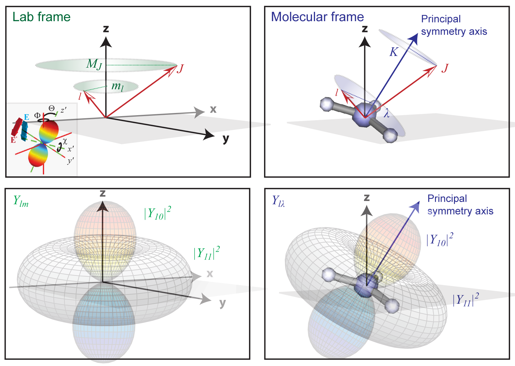
Fig. 3.1 Reference frame and angular momentum definitions for the Laboratory frame (LF) and Molecular frame (MF), using a general notation from molecular spectroscopy. In this case the LF shows an angular momentum vectors \(J\) and \(l\); \(J\) is usually used to define rotational (or sometimes total) angular momentum of the system, and \(l\) the electronic component. Projection terms onto the LF \(z\)-axis, \(M_J\) and \(m_l\) are also indicated. In the MF equivalent angular momentum terms are shown, with projections \(K\) and \(\lambda\) onto the molecular symmetry axis. The insert shows a frame rotation \((x,y,z)\leftarrow(x',y',z')\), defined by a set of Euler angles \(R_{\hat{n}}=\{\chi,\Theta,\Phi\}\), and illustrating the rotation of the \(z\)-axis (defined by the electric field vector \(E\)), and a spherical harmonic function in the \((x',y',z')\) frame. See also Fig. 1.1. Figure reproduced from Quantum Metrology Vol. 1 [4], Fig. 2.3 - note that some alternative notations are used in this volume.

3.3.4. Numerical aside: symmetry-defined channel functions

In the following sub-sections, each component is defined in detail, including numerical examples. For illustration purposes, the numerical example uses a minimal set of assumptions, and is defined initially purely by symmetry, although further terms may be required for computation of some of the geometric terms and are discussed where required. A fuller discussion of symmetry considerations in photoionization can be found in Sect. 3.2, and discussion of symmetrized harmonics in Sect. 3.6.2.

For this example, the \(D_{2h}\) point group is used, representing a fairly general case of a planar asymmetric top system, e.g. ethylene (\(C_2H_4\)). Note that, in this case, the symmetrization coefficients (\(b_{hl\lambda}^{\Gamma\mu}\), see Eqn. (3.38)) have the property that \(\mu=0\) only, and the \(h\) index is redundant, since it maps uniquely to \(l\) - see Fig. 3.2 - so these indexes can be dropped. Note, also, the unfortunate convention that the label \(\mu\) is used for multiple indexes; to avoid ambiguity this term is remapped to \(\mu_X\) in the numerics below. However, in this case, since \(\mu\) can be dropped from the symmetrization coefficients, there is actually no ambiguity in later usage.

Note

Full tabulations of the parameters available in HTML or notebook formats only.

Show code cell content Hide code cell content

# Run default config - may need to set full path here
%run '../scripts/setup_notebook.py'

# Override plotters backend?
# plotBackend = 'pl'

# Set Matplotlib inline for lmPlot() with Seaborn display
%matplotlib inline

*** Setting up notebook with standard Quantum Metrology Vol. 3 imports...
For more details see https://pemtk.readthedocs.io/en/latest/fitting/PEMtk_fitting_basic_demo_030621-full.html
To use local source code, pass the parent path to this script at run time, e.g. "setup_fit_demo ~/github"

*** Running: 2023-12-07 10:45:06
Working dir: /home/jovyan/jake-home/buildTmp/_latest_build/html/doc-source/part1
Build env: html
None

* Loading packages...
* sparse not found, sparse matrix forms not available. 
* natsort not found, some sorting functions not available. 
* Setting plotter defaults with epsproc.basicPlotters.setPlotters(). Run directly to modify, or change options in local env.
* Set Holoviews with bokeh.
* pyevtk not found, VTK export not available. 
* Set Holoviews with bokeh.
Jupyter Book      : 0.15.1
External ToC      : 0.3.1
MyST-Parser       : 0.18.1
MyST-NB           : 0.17.2
Sphinx Book Theme : 1.0.1
Jupyter-Cache     : 0.6.1
NbClient          : 0.7.4

#*** Setup symmetry-defined matrix elements using PEMtk

# Import class
from pemtk.sym.symHarm import symHarm

#*** Compute hamronics for Td, lmax=4
sym = 'D2h'
lmax=4

lmaxPlot = 2  # Set lmaxPlot for subselection on plots later.

# Create symHarm object with given settings, 
# this will also compute the symmetrized harmonics
symObj = symHarm(sym,lmax)

Show code cell output Hide code cell output

*** Mapping coeffs to ePSproc dataType = matE
Remapped dims: {'C': 'Cont', 'mu': 'it'}
Added dim Eke
Added dim Targ
Added dim Total
Added dim mu
Added dim Type
Found dipole symmetries: 
{'B1u': {'m': [0], 'pol': ['z']}, 'B2u': {'m': [-1, 1], 'pol': ['y']}, 'B3u': {'m': [-1, 1], 'pol': ['x']}}

Show code cell content Hide code cell content

# Glue items for later
glue("symHarmPGmatE", sym, display=False)
glue("symHarmLmaxmatE", lmax, display=False)
glue("symHarmBasislmaxPlot", lmaxPlot, display=False)

# Display results (real harmonics)
symObj.displayXlm(setCols='h')  #, dropLevels='mu')

# Glue version for JupyterBook output
# As above, but with PD object return and glue.
glue("D2hXlm",symObj.displayXlm(setCols='h',returnPD=True), display=False)

Show code cell output Hide code cell output

				b
			h	0	1	2	3	4	5
Character ($\Gamma$)	PFIX ($\mu$)	l	m
A1g	0	0	0	1.0
		2	0		1.0
			2			1.0
		4	0				1.0
			2					1.0
			4						1.0
A1u	0	3	-2	1.0
B1g	0	2	-2	1.0
		4	-4		1.0
			-2			1.0
B1u	0	1	0	1.0
		3	0		1.0
			2			1.0
B2g	0	2	1	1.0
		4	1		1.0
			3			1.0
B2u	0	1	-1	1.0
		3	-3		1.0
			-1			1.0
B3g	0	2	-1	1.0
		4	-3		1.0
			-1			1.0
B3u	0	1	1	1.0
		3	1		1.0
			3			1.0

				b
			h	0	1	2	3	4	5
Character ($\Gamma$)	PFIX ($\mu$)	l	m
A1g	0	0	0	1.0
		2	0		1.0
			2			1.0
		4	0				1.0
			2					1.0
			4						1.0
A1u	0	3	-2	1.0
B1g	0	2	-2	1.0
		4	-4		1.0
			-2			1.0
B1u	0	1	0	1.0
		3	0		1.0
			2			1.0
B2g	0	2	1	1.0
		4	1		1.0
			3			1.0
B2u	0	1	-1	1.0
		3	-3		1.0
			-1			1.0
B3g	0	2	-1	1.0
		4	-3		1.0
			-1			1.0
B3u	0	1	1	1.0
		3	1		1.0
			3			1.0

Fig. 3.2 Symmetrized harmonics coefficients (\(b_{hl\lambda}^{\Gamma\mu}\), see Eqn. (3.38)) for D2h symmetry (\(l_{max}=\)4) generated with the Photoelectron Metrology Toolkit [5] wrapper for libmsym [64, 65]. Note that, in this case, the coeffcients have the property that \(\mu=0\) only, and the \(h\) index is redundant (maps uniquely to \(l\)).

To compute basis tensors from these symmetry coefficients, they can be converted to the standard radial matrix elements format used in the Photoelectron Metrology Toolkit [5] (see Sect. 6.3.4 for further discussion of the numerical implementation), and used with the standard routines. These are demonstrated below, for two flavours - the base ePSproc [34] routine for computation of AF-PADs, and the Photoelectron Metrology Toolkit [5] fitting routine which wraps this functionality. Note that all tensors are stored as Xarray [53, 54] objects, which allow for easy numerical manipulation, subselection etc.

#*** Compute basis functions for given matrix elements using PEMtk fit class
# This illustration uses the symmetrized matrix elements set above

#*** To use ePSproc/PEMtk classes, 
# these values can be converted to ePSproc BLM data type...
# Run conversion - the default is to set the coeffs to the 'BLM' data type, 
# additional dim mappings can also be set.
# Outputs are set to symObj.coeffs[dataType]
dimMap = {'C':'Cont','mu':'muX'}
symObj.toePSproc(dimMap=dimMap)

# Run conversion with a different dimMap & dataType
# Outputs are set to symObj.coeffs[dataType]
dataType = 'matE'
symObj.toePSproc(dimMap = dimMap, dataType=dataType)


#*** Setup class object
data = pemtkFit()

# Set to new key in data class
dataKey = sym
data.data[dataKey] = {}

# Set data.data[dataKey][dataType] from cases set above
# This pushes the symmetrized coeffs computed above to the PEMtk fit class 
# object for general use with PEMtk methods.
# Here set 'matE' for use as matrix elements, and 'BLM' for pad plotting routines.
for dataType in ['matE','BLM']:
    # Select expansion in complex harmonics, and sum redundant dims
    data.data[dataKey][dataType] = symObj.coeffs[dataType]['b (comp)'].sum(['h','muX']) 
    # Propagate attrs
    data.data[dataKey][dataType].attrs = symObj.coeffs[dataType].attrs

# Set data by key
# data.subKey is the default location used by the PEMtk routines
data.subKey = dataKey


#*** Compute basis function - two flavours
# Using PEMtk `afblmMatEfit` method 
# - this only returns the product basis set as used for fitting
# See the docs for more details, https://pemtk.readthedocs.io
phaseConvention='S'  # For consistency in the method, explicitly set the
                     # phase convention used here ('S' = standard, 'E' = ePS).
BetaNormX, basisProduct = data.afblmMatEfit(selDims={}, 
                                            sqThres=False, 
                                            phaseConvention=phaseConvention)

# Using ePSproc directly - this includes full basis return if specified
# See the docs for more details, https://epsproc.readthedocs.io
BetaNormX2, basisFull = ep.geomFunc.afblmXprod(data.data[data.subKey]['matE'], 
                                               basisReturn = 'Full', 
                                               thres=None, selDims={}, 
                                               sqThres=False,
                                               phaseConvention=phaseConvention)

# The basis dictionary contains various numerical parameters, these are investigated below.
# See also the ePSproc docs at 
# https://epsproc.readthedocs.io/en/latest/methods/geometric_method_dev_260220_090420_tidy.html
print(f"Product basis elements: {basisProduct.keys()}")
print(f"Full basis elements: {basisFull.keys()}")

# Use full basis for following sections
basis = basisFull

*** Mapping coeffs to ePSproc dataType = BLM
Remapped dims: {'C': 'Cont', 'mu': 'muX'}
Added dim Eke
Added dim P
Added dim T
Added dim C
*** Mapping coeffs to ePSproc dataType = matE
Remapped dims: {'C': 'Cont', 'mu': 'muX'}
Added dim Eke
Added dim Targ
Added dim Total
Added dim mu
Added dim it
Added dim Type
Product basis elements: dict_keys(['BLMtableResort', 'polProd', 'phaseConvention', 'BLMRenorm'])
Full basis elements: dict_keys(['QNs', 'EPRX', 'lambdaTerm', 'BLMtable', 'BLMtableResort', 'AFterm', 'AKQS', 'polProd', 'phaseConvention', 'BLMRenorm', 'matEmult'])

3.3.5. Matrix element geometric coupling term \(B_{L,M}\)

The coupling of the partial-waves as coherent pairs, \(|l,m\rangle\) and \(|l',m'\rangle\), into the observable set of \(\{L,M\}\) is defined by a tensor contraction with two 3j terms:

(3.20)\[\begin{split} B_{L,M}=(-1)^{m}\left(\frac{(2l+1)(2l'+1)(2L+1)}{4\pi}\right)^{1/2}\left(\begin{array}{ccc} l & l' & L\\ 0 & 0 & 0 \end{array}\right)\left(\begin{array}{ccc} l & l' & L\\ -m & m' & M \end{array}\right) \end{split}\]

Note that this term is equivalent, effectively, to a triple integral over spherical harmonics (e.g. Eq. 3.119 in Zare [83]):

\[\begin{split} \begin{aligned} \intop_{0}^{2\pi}\intop_{0}^{\pi}Y_{J_{3}M_{3}}(\theta,\phi)Y_{J_{2}M_{2}}(\theta,\phi)Y_{J_{1}M_{1}}(\theta,\phi)\sin\theta d\theta d\phi & = & \left(\frac{(2J_{1}+1)(2J_{2}+1)(2J_{3}+1)}{4\pi}\right)^{1/2}\\ & \times & \left(\begin{array}{ccc} J_{1} & J_{2} & J_{3}\\ 0 & 0 & 0 \end{array}\right)\left(\begin{array}{ccc} J_{1} & J_{2} & J_{3}\\ M_{1} & M_{2} & M_{3} \end{array}\right) \end{aligned} \end{split}\]

And a similar term appears in the contraction over a pair of harmonics into a resultant harmonic (e.g. Eqs. C.21, C.22 in Blum [97]) - this is how the term arises in the derivation of the observables.

\[\begin{split} \begin{aligned} Y_{J_{1}M_{1}}(\theta,\phi)Y_{J_{2}M_{2}}(\theta,\phi) & = & \sum_{J_{3}M_{3}}\left(\frac{(2J_{1}+1)(2J_{2}+1)(2J_{3}+1)}{4\pi}\right)^{1/2}\\ & \times & \left(\begin{array}{ccc} J_{1} & J_{2} & J_{3}\\ 0 & 0 & 0 \end{array}\right)\left(\begin{array}{ccc} J_{1} & J_{2} & J_{3}\\ M_{1} & M_{2} & M_{3} \end{array}\right)Y_{J_{3}M_{3}}^{*}(\theta,\phi) \end{aligned} \end{split}\]

Note also some definitions use conjugate spherical harmonics, which can be converted as, e.g., Eq. C.21 in Blum [97]:

(3.21)\[\begin{equation} \beta_{L,M}^{\mu_{i},\mu_{f}}Y_{LM}^{*}(\theta_{\hat{k}},\phi_{\hat{k}})=\beta_{L,-M}^{\mu_{i},\mu_{f}}(-1)^{M}Y_{L,-M}(\theta_{\hat{k}},\phi_{\hat{k}})\label{eq:sph-conj-conv} \end{equation}\]

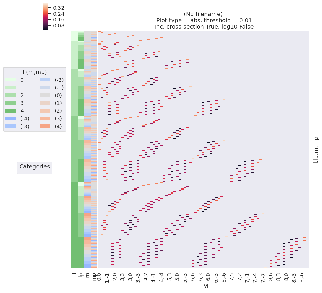
In the current Photoelectron Metrology Toolkit [5] codebase, the relevant basis item can be inspected as below, in order to illustrate the sensitivity of different \((L,M)\) terms to the matrix element products. In many typical cases, however, this term is restricted to only \(M=0\) components overall by other geometric factors (see below).

The code cells below illustrate this for the current example case, and Fig. 3.3 offers a general summary. In general, this is a convenient way to visualize the selection rules into the observable: for instance, only terms \(l=l'\) and \(m=-m'\) contribute to the overall photoionization cross-section term (\(L=0, M=0\)), and the maximum observable \(L_{max}=2l_{max}\). However, since these terms are fairly simply followed algebraically in this case, via the rules inherent in the \(3j\) product (Eq. (3.20)), this is not particularly insightful (although useful pedagogically). These visualizations will become more useful when dealing with real sets of matrix elements, and specific polarization geometries, which will further modulate or restrict the \(B_{L,M}\) terms.

Numerically, various standard functions may be used to quickly gain deeper insight, for example min/max, averages etc. Such considerations may provide a quick sanity-check for a given case, and may prove useful when planning experiments to investigate particular aspects or channels of a given system. Other properties of the basis functions may also be interrogated numerically; for instance, correlation maps provide an alternative way to check which terms are strongly correlated or coupled, or will dominate a given aspect of the observable.

#*** Tabulate basis

basisKey = 'BLMtableResort'  # Key for BLM basis set

# Reformat basis for display (optional)
stackDims = {'LM':['L','M']}
basisPlot = basis[basisKey].rename({'S-Rp':'M'}).stack(stackDims)

# Convert to Pandas, use ep.multiDimXrToPD as a general multi-dimensional restacker
pd, _ = ep.multiDimXrToPD(basisPlot, colDims=stackDims)

# Summarise properties and tabulate via Pandas Describe
pd.describe().T

Show code cell output Hide code cell output

		count	mean	std	min	25%	50%	75%	max
L	M
0	0	25.0	0.011	2.877e-01	-0.282	-0.282	0.282	0.282	0.282
1	1	32.0	0.005	2.265e-01	-0.326	-0.173	0.011	0.206	0.320
	0	32.0	0.007	2.265e-01	-0.238	-0.222	0.011	0.221	0.282
	-1	32.0	0.005	2.265e-01	-0.326	-0.173	0.011	0.206	0.320
2	2	34.0	0.021	2.047e-01	-0.320	-0.180	0.040	0.185	0.337
	1	38.0	0.018	1.935e-01	-0.261	-0.162	0.059	0.216	0.282
	0	42.0	0.015	1.841e-01	-0.229	-0.180	0.057	0.167	0.282
	-1	38.0	0.018	1.935e-01	-0.261	-0.162	0.059	0.216	0.282
	-2	34.0	0.021	2.047e-01	-0.320	-0.180	0.040	0.185	0.337
3	3	26.0	0.026	2.090e-01	-0.326	-0.140	0.077	0.188	0.320
	2	32.0	0.031	1.865e-01	-0.282	-0.125	0.070	0.192	0.282
	1	38.0	0.032	1.701e-01	-0.238	-0.149	0.083	0.183	0.282
	0	38.0	0.033	1.700e-01	-0.195	-0.099	-0.044	0.195	0.282
	-1	38.0	0.032	1.701e-01	-0.238	-0.149	0.083	0.183	0.282
	-2	32.0	0.031	1.865e-01	-0.282	-0.125	0.070	0.192	0.282
	-3	26.0	0.026	2.090e-01	-0.326	-0.140	0.077	0.188	0.320
4	4	19.0	0.065	2.147e-01	-0.229	-0.166	0.107	0.248	0.337
	3	26.0	0.054	1.825e-01	-0.204	-0.159	0.096	0.188	0.282
	2	33.0	0.046	1.621e-01	-0.190	-0.084	0.066	0.191	0.282
	1	36.0	0.044	1.547e-01	-0.201	-0.140	0.079	0.168	0.282
	0	39.0	0.042	1.486e-01	-0.190	-0.073	0.040	0.160	0.282
	-1	36.0	0.044	1.547e-01	-0.201	-0.140	0.079	0.168	0.282
	-2	33.0	0.046	1.621e-01	-0.190	-0.084	0.066	0.191	0.282
	-3	26.0	0.054	1.825e-01	-0.204	-0.159	0.096	0.188	0.282
	-4	19.0	0.065	2.147e-01	-0.229	-0.166	0.107	0.248	0.337
5	5	10.0	0.112	2.433e-01	-0.190	-0.139	0.212	0.329	0.347
	4	16.0	0.090	1.876e-01	-0.208	-0.015	0.145	0.232	0.295
	3	22.0	0.072	1.608e-01	-0.196	-0.069	0.127	0.199	0.260
	2	26.0	0.063	1.490e-01	-0.179	-0.065	0.085	0.190	0.246
	1	30.0	0.055	1.398e-01	-0.161	-0.092	0.093	0.173	0.241
	0	30.0	0.055	1.397e-01	-0.171	-0.076	0.054	0.166	0.246
	-1	30.0	0.055	1.398e-01	-0.161	-0.092	0.093	0.173	0.241
	-2	26.0	0.063	1.490e-01	-0.179	-0.065	0.085	0.190	0.246
	-3	22.0	0.072	1.608e-01	-0.196	-0.069	0.127	0.199	0.260
	-4	16.0	0.090	1.876e-01	-0.208	-0.015	0.145	0.232	0.295
	-5	10.0	0.112	2.433e-01	-0.190	-0.139	0.212	0.329	0.347
6	6	6.0	0.160	2.560e-01	-0.163	-0.069	0.285	0.354	0.360
	5	10.0	0.130	1.863e-01	-0.200	0.100	0.204	0.255	0.289
	4	14.0	0.107	1.571e-01	-0.191	0.004	0.166	0.230	0.266
	3	18.0	0.090	1.405e-01	-0.156	0.048	0.109	0.179	0.252
	2	22.0	0.077	1.294e-01	-0.165	0.004	0.090	0.177	0.243
	1	24.0	0.072	1.247e-01	-0.160	0.007	0.099	0.152	0.230
	0	26.0	0.066	1.210e-01	-0.156	0.007	0.062	0.174	0.239
	-1	24.0	0.072	1.247e-01	-0.160	0.007	0.099	0.152	0.230
	-2	22.0	0.077	1.294e-01	-0.165	0.004	0.090	0.177	0.243
	-3	18.0	0.090	1.405e-01	-0.156	0.048	0.109	0.179	0.252
	-4	14.0	0.107	1.571e-01	-0.191	0.004	0.166	0.230	0.266
	-5	10.0	0.130	1.863e-01	-0.200	0.100	0.204	0.255	0.289
	-6	6.0	0.160	2.560e-01	-0.163	-0.069	0.285	0.354	0.360
7	7	2.0	0.369	0.000e+00	0.369	0.369	0.369	0.369	0.369
	6	4.0	0.260	2.159e-02	0.242	0.242	0.260	0.279	0.279
	5	6.0	0.208	5.293e-02	0.150	0.164	0.205	0.252	0.268
	4	8.0	0.174	6.729e-02	0.087	0.130	0.178	0.222	0.251
	3	10.0	0.149	7.566e-02	0.045	0.098	0.148	0.214	0.239
	2	12.0	0.129	8.089e-02	0.020	0.062	0.130	0.195	0.239
	1	14.0	0.114	8.427e-02	0.007	0.038	0.124	0.198	0.225
	0	14.0	0.114	8.308e-02	0.018	0.034	0.082	0.183	0.236
	-1	14.0	0.114	8.427e-02	0.007	0.038	0.124	0.198	0.225
	-2	12.0	0.129	8.089e-02	0.020	0.062	0.130	0.195	0.239
	-3	10.0	0.149	7.566e-02	0.045	0.098	0.148	0.214	0.239
	-4	8.0	0.174	6.729e-02	0.087	0.130	0.178	0.222	0.251
	-5	6.0	0.208	5.293e-02	0.150	0.164	0.205	0.252	0.268
	-6	4.0	0.260	2.159e-02	0.242	0.242	0.260	0.279	0.279
	-7	2.0	0.369	0.000e+00	0.369	0.369	0.369	0.369	0.369
8	8	1.0	0.380	NaN	0.380	0.380	0.380	0.380	0.380
	7	2.0	0.269	5.551e-17	0.269	0.269	0.269	0.269	0.269
	6	3.0	0.215	5.424e-02	0.184	0.184	0.184	0.231	0.277
	5	4.0	0.180	6.937e-02	0.120	0.120	0.180	0.240	0.240
	4	5.0	0.155	7.763e-02	0.075	0.075	0.189	0.189	0.249
	3	6.0	0.136	8.257e-02	0.043	0.066	0.136	0.205	0.228
	2	7.0	0.120	8.559e-02	0.022	0.056	0.090	0.188	0.238
	1	8.0	0.107	8.742e-02	0.010	0.042	0.097	0.161	0.222
	0	9.0	0.095	8.852e-02	0.003	0.027	0.094	0.188	0.234
	-1	8.0	0.107	8.742e-02	0.010	0.042	0.097	0.161	0.222
	-2	7.0	0.120	8.559e-02	0.022	0.056	0.090	0.188	0.238
	-3	6.0	0.136	8.257e-02	0.043	0.066	0.136	0.205	0.228
	-4	5.0	0.155	7.763e-02	0.075	0.075	0.189	0.189	0.249
	-5	4.0	0.180	6.937e-02	0.120	0.120	0.180	0.240	0.240
	-6	3.0	0.215	5.424e-02	0.184	0.184	0.184	0.231	0.277
	-7	2.0	0.269	5.551e-17	0.269	0.269	0.269	0.269	0.269
	-8	1.0	0.380	NaN	0.380	0.380	0.380	0.380	0.380

#*** Plot BLM terms for basis set - basic case
basisKey = 'BLMtableResort'

# Basic plot
ep.lmPlot(basisPlot, xDim=stackDims);  # Basic plot with all terms

Show code cell output Hide code cell output

Plotting data (No filename), pType=a, thres=0.01, with Seaborn

No artists with labels found to put in legend.  Note that artists whose label start with an underscore are ignored when legend() is called with no argument.

#*** Plot BLM terms for basis set - plot with some additional figure formatting options

# Formatting options
titleString=f'$B_{{L,M}}$ terms for {sym}, lmax={lmaxPlot}'
titleDetails=True
labelRound = 1
catLegend=False
labelCols = [1,1]

# cmap = None for default.
# cmap = 'vlag'

# lmPlot with various options
*_, gFig = ep.lmPlot(basisPlot.where((basisPlot.l<=lmaxPlot) 
                        & (basisPlot.lp<=lmaxPlot)), 
                       xDim=stackDims, pType = 'r', 
                       cmap=cmap, labelRound = labelRound, 
                       catLegend=catLegend, 
                       titleString=titleString, titleDetails=titleDetails, 
                       labelCols = labelCols);

# Glue figure
glue("lmPlot_BLM_basis_D2h", gFig.fig, display=False)

Show code cell output Hide code cell output

Plotting data (No filename), pType=r, thres=0.01, with Seaborn

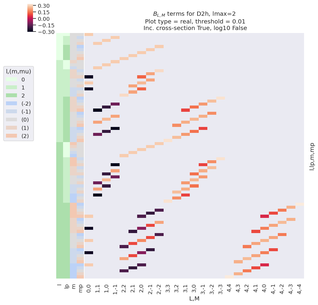
Fig. 3.3 Example \(B_{L,M}\) basis functions for D2h symmetry. Note figure is truncated to \(l_{max}=l'_{max}=\)2 for clarity. The colour-map (top left) shows the (real) values of the allowed terms shown in the main panel of the figure. The key (middle left) indicates categorical colour-mapping for the \((l,l',m,m')\) terms corresponding to the left-hand side-panel of the main plot, which illustrates the quantum numbers for each row.

3.3.6. Electric field geometric coupling term \({E_{P,R}(\hat{e};\mu_{0})}\)

The coupling of two 1-photon terms (which arises in the square of the ionization matrix element as per Eq. (3.9)) can be written as a tensor contraction:

(3.22)\[\begin{split} E_{P,R}(\hat{e})=[e\otimes e^{*}]_{R}^{P}=[P]^{\frac{1}{2}}\sum_{p}(-1)^{R}\left(\begin{array}{ccc} 1 & 1 & P\\ p & R-p & -R \end{array}\right)e_{p}e_{R-p}^{*} \end{split}\]

Where:

• \(e_{p}\) and \(e_{R-p}\) define the field strengths for the polarizations \(p\) and \(R-p\), which are coupled into the spherical tensor \(E_{PR}\);

• square-brackets indicate degeneracy terms, e.g. \([P]^{\frac{1}{2}} = (2P+1)^{\frac{1}{2}}\);

• in the literature LF/AF field projection terms are usually denoted \(p\) (as above) or \(\mu_0\) (used as a more general angular-momentum projection notation). For the MF case photon projection terms are usually denoted by \(q\) or \(\mu\).

• The polarization vector or propagation direction is usually chosen to define the LF/AF z-axis for linear or non-linearly polarized light respectively (see Fig. 1.1 for the linear example), or defined relative to the molecular symmetry axis in the MF. (See Sect. 3.3.3 for further details.)

• For a given case the polarization geometry may define a single projection term, or there may be multiple terms allowed. For instance, linearly polarized light is defined by \(\mu_0=0\) only, resulting in non-zero values for just the \(P=0,2\) terms in Eq. (3.22), i.e. product terms \(E_{0,0}, E_{2,0}\) are allowed. Non-linearly polarized light may contain all allowed components (\(\mu_0=-1,0,1\)). For the MF case, allowed components may be defined directly in the MF or determined via a frame transformation from the LF - see Sect. 3.3.7.

• Note this notation implicitly describes only the time-independent photon angular momentum coupling, but time-dependent/shaped laser fields can be readily incorporated by allowing for time-dependent fields \(e_{p}(t)\) (see, for instance, Ref. [99]). (Support for this is planned in ePSproc [34], as of v1.3.2 this is in the development and testing phase.)

To derive this result, one can start from a general spherical tensor direct product, e.g., Eq. 5.36 in Zare [83]; for two first-rank tensors (e.g. electric field vectors) this contraction is given explicitly by Eq. 5.40 in Zare [83]:

(3.23)\[\begin{equation} [A^{(1)}\otimes B^{(1)}]_{q}^{k}=\sum_{m}\langle1m,1q-m|kq\rangle A(1,m)B(1,q-m) \end{equation}\]

This can be converted to \(3j\) form:

(3.24)\[\begin{equation} [A^{(1)}\otimes B^{(1)}]_{q}^{k}=\sum_{m}(-1)^{q}[k]^{1/2}\left(\begin{array}{ccc} 1 & 1 & k\\ m & q-m & -q \end{array}\right)A(1,m)B(1,q-m) \end{equation}\]

And the appropriate E-field terms substituted in to arrive at equation Eq. (3.22).

As before, we can visualise these values with the Photoelectron Metrology Toolkit [5], as illustrated in the following code block, and corresponding output Fig. 3.4.

#*** For illustration, recompute EPR term for default case.
EPRX = ep.geomCalc.EPR(form = 'xarray')

# Set parameters to restack the Xarray into (L,M) pairs
plotDimsRed = ['p', 'R-p']
xDim = {'PR':['P','R']}

# Plot with ep.lmPlot(), real values
*_, gFig = ep.lmPlot(EPRX, plotDims=plotDimsRed, xDim=xDim, 
                     pType = 'r', 
                     titleString=f'$E_{{P,R}}$ terms (all cases).',
                     labelCols = labelCols)

# Alternative version summed over l,l',m
# *_, gFig = ep.lmPlot(EPRX.unstack().sum(['l','lp','R-p']), xDim=xDim, pType = 'r')

# Glue figure
glue("lmPlot_EPR_basis", gFig.fig)

Show code cell output Hide code cell output

Plotting data (No filename), pType=r, thres=0.01, with Seaborn

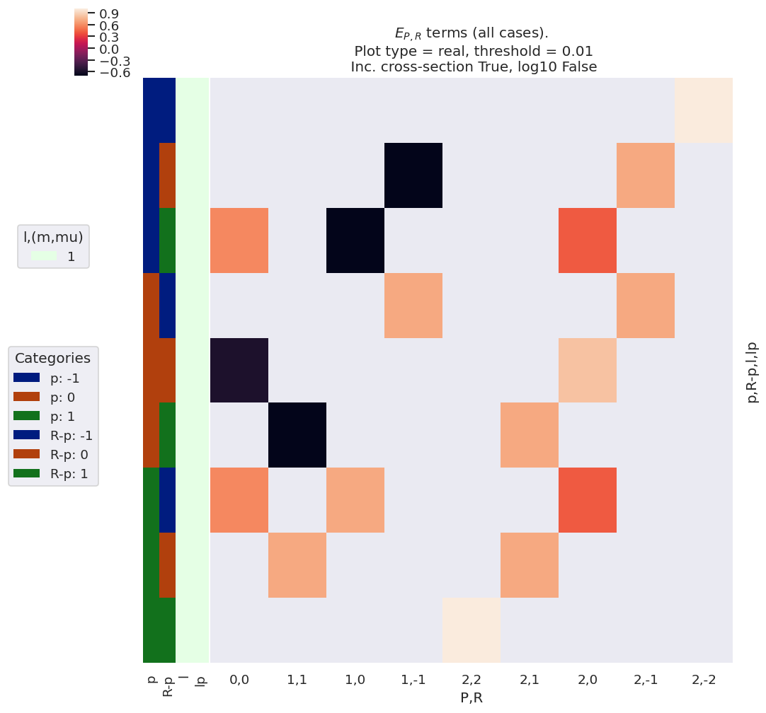
Fig. 3.4 Example \(E_{P,R}\) basis functions. Note that for linearly polarised light \(p=R-p=0\) only, hence only the terms \(E_{0,0}\) and \(E_{2,0}\) are non-zero in this case. For non-linearly polarised cases many other terms are allowed. The colour-map (top left) shows the (real) values of the allowed terms shown in the main panel of the figure. The first key (middle left) indicates categorical colour-mapping for the \((l,l')\) terms (and \(l=l'=1\) only in this case), and the second (“Categories”) key indicates the colour-mapping for the remaining terms. The keys correspond to the left-hand side-panel of the main plot, which indicates the quantum numbers for each row.

3.3.7. Molecular frame projection term \(\Lambda\)

For the molecular frame case, the coupling between the LF and MF can be defined by a projection term, \(\Lambda_{R',R}(R_{\hat{n}})\):

(3.25)\[\begin{split} \Lambda_{R',R}(R_{\hat{n}})=(-1)^{(R')}\left(\begin{array}{ccc} 1 & 1 & P\\ \mu & -\mu' & R' \end{array}\right)D_{-R',-R}^{P}(R_{\hat{n}}) \end{split}\]

This is similar to the \(E_{P,R}\) term, and essentially rotates it into the MF, defining the projections of the polarization vector (photon angular momentum) \(\mu\) into the MF for a given molecular orientation (frame rotation) defined by a set of rotations. The frame rotation is parameterized by a set of Euler angles, \(R_{\hat{n}}=\{\chi,\Theta,\Phi\}\), with projections given by Wigner rotation matrix elements \(D_{-R',-R}^{P}(R_{\hat{n}})\).

For the LF/AF case, the same term appears but in a simplified form:

(3.26)\[\begin{split} \bar{\Lambda}_{R'}=(-1)^{(R')}\left(\begin{array}{ccc} 1 & 1 & P\\ \mu & -\mu' & R' \end{array}\right)\equiv\Lambda_{R',R'}(R_{\hat{n}}=0) \end{split}\]

This form pertains since - in the LF/AF case - there is no specific frame transformation defined (i.e. there is no single molecular orientation defined in relation to the light polarization, rather a distribution as defined by the ADMs), but the total angular momentum coupling of the photon terms is still required in the equations.

Numerically, the function is calculated for a specified set of orientations, which default to the standard set of \((x,y,z)\) MF polarization cases in the Photoelectron Metrology Toolkit [5] routines. For the LF/AF case, this term is still used, but restricted to \(R_{\hat{n}} = (0,0,0) = z\), i.e. no frame rotation relative to the LF \(E_{P,R}\) definition. In some cases additional frame transformations may be required here to define, e.g., the use of the propagation axis as the reference \(z\)-axis for circularly or elliptically polarized light. (See Sect. 3.3.3 for further discussion.)

3.3.8. Alignment tensor \(\Delta_{L,M}(K,Q,S)\)

Finally, for the LF/AF case, the alignment tensor couples the molecular axis ensemble (defined as a set of ADMs, see Sect. 3.5 for details) and the photoionization multipole terms into the final observable.

(3.27)\[\begin{split} \Delta_{L,M}(K,Q,S)=(2K+1)^{1/2}(-1)^{K+Q}\left(\begin{array}{ccc} P & K & L\\ R & -Q & -M \end{array}\right)\left(\begin{array}{ccc} P & K & L\\ R' & -S & S-R' \end{array}\right) \end{split}\]

In the full equations for the observable, this term appears in a summation with the ADMs, as:

(3.28)\[ \tilde{\Delta}_{L,M}(t) = \sum_{K,Q,S}\Delta_{L,M}(K,Q,S)A_{Q,S}^{K}(t) \]

This summed alignment term can be considered, essentially, as a (coherent) geometric averaging of the MF observable weighted by the axis distribution in the AF (for more on the axis averaging as a convolution, see Refs. [4, 96]); equivalently, the averaging can be considered as a purely angular-momentum coupling effect, which accounts for all contributing moments of the various aspects of the system, and defines the allowed projections onto the final observables in the LF.

Mappings of these terms are investigated numerically below, for some examplar cases.

3.3.8.1. Basic cases

Fig. 3.5 illustrates the alignment tensor \(\Delta_{L,M}(K,Q,S)\) for some basic cases, and values are also tabulated in Table 3.6. Note that for illustration purposes the term is subselected with \(K=0\), \(Q=0\), \(S=0\) and \(R'=0\); \(R\neq0\) terms are included to illustrate the elliptically-polarized case, which can give rise to non-zero \(M\) terms.

For the simplest case of an unaligned ensemble, this term is restricted to \(K=Q=S=0\), i.e. \(\Delta_{L,M}(0,0,0)\); for single-photon ionization with linearly-polarized light (\(p=0\), hence \(P=0,2\) and \(R=R'=0\)), this has non-zero values for \(L=0,2\) and \(M=0\) only. Typically, this simplest case is synonymous with standard LF results, and maintains cylindrical and up-down symmetry in the observable.

For circularly polarized light (\(p=\pm1\), hence \(P=0,1,2\) and \(R=R'=0\)), odd-\(L\) is allowed, signifying up/down symmetry breaking in the observable (where up/down pertains to the propagation direction of the light, conventionally the \(z\)-axis for non-linear polarizations, see Sect. 3.3.3). For elliptically polarized light, mixing of terms with different \(p\) allows for non-zero \(R\) terms (see Eq. (3.22)), hence non-zero \(M\) is allowed (see Eq. (3.27)), signifying breaking of cylindrical symmetry in the observable is allowed. Note, however, that non-zero values here do not indicate that such effects will be observed in any given case, only that they may be (or, at least, are not restricted by the alignment tensor).

#*** Set range of ADMs for test as time-dependent values (linear ramps)

# Set ADMs for increasing alignment...
# Note that delta term is independent of the absolute values of the ADMs(t), 
# but does use this term to define limits on some quantum numbers.

tPoints = 10  # 10 t-points
inputADMs = [[0,0,0, *np.ones(tPoints)],
             [2,0,0, *np.linspace(0,1,tPoints)], 
             [4,0,0, *np.linspace(0,0.5,tPoints)],
             [6,0,0, *np.linspace(0,0.3,tPoints)],
             [8,0,0, *np.linspace(0,0.2,tPoints)]]

# Set to AKQS parameters in Xarray
AKQS = ep.setADMs(ADMs = inputADMs)

# Use default EPR term - note this computes for all pol states, p=[-1,0,1]
EPR = ep.geomCalc.EPR(form='xarray')

#*** Compute alignment terms
AFterm, DeltaTerm = ep.geomCalc.deltaLMKQS(EPR, AKQS)

#*** Plot Delta term with subselections and formatting
xDim = {'LM':['L','M']}
daPlot, daPlotpd, legendList, gFig = ep.lmPlot(
                     DeltaTerm.sel(K=0,Q=0,S=0,Rp=0).sel({'S-Rp':0}), 
                     xDim = xDim, 
                     pType = 'r', squeeze = False, thres=None,
                     titleString="$\Delta(0,0,0)$ term ($R'=0$ only)",
                     # Set dim mapping to use P,R with "l,m" colourmap
                     dimMaps={'lDims':['P'],'mDims':'R'},  
                     labelCols=labelCols,
                     catLegend=False)


# Glue versions for JupyterBook output
glue("deltaTerm000-lmPlot", gFig.fig, display=False)
# As above, but with PD object return and glue.
glue("deltaTerm000-tab",daPlotpd.fillna(''), display=False)  

Show code cell output Hide code cell output

Set dataType (No dataType)
Plotting data (No filename), pType=r, thres=None, with Seaborn

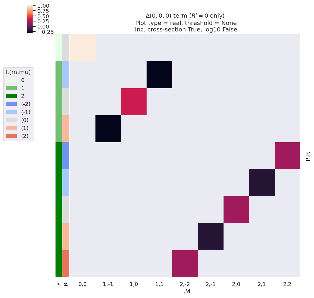
Fig. 3.5 Example \(\Delta_{L,M}(0,0,0)\) basis functions (see also Fig. 3.6). For illustration purposes, the plot only shows terms for \(R'=0\). See main text for discussion.

	L	0	1			2
	M	0	-1	0	1	-2	-1	0	1	2
P	R
0	0	1.0
1	-1				-0.333
	0			0.333
	1		-0.333
2	-2									0.2
	-1								-0.2
	0							0.2
	1						-0.2
	2					0.2

Fig. 3.6 Example \(\Delta_{L,M}(0,0,0)\) basis functions (see also Fig. 3.5). For illustration purposes, the table only shows terms for \(R'=0\). See main text for discussion.

#*** Plot ADMs
*_, ADMFig = ep.lmPlot(AKQS, xDim = 't', pType = 'r', 
                       labelCols=labelCols, catLegend=False,
                       cmap='vlag',
                       titleString='ADMs (linear ramp example)') 

#*** Plot AF term with subselection
*_, AFFig = ep.lmPlot(AFterm.sel(R=0).sel(Rp=0).sel({'S-Rp':0}), 
                      xDim = 't', pType = 'r', 
                      labelCols=labelCols,
                      cmap='vlag',
                      titleString='$\\tilde{\Delta}_{L,M}(t)$ (linear ramp example)') 

# Glue versions for JupyterBook output
glue("ADMs-linearRamp-lmPlot", ADMFig.fig, display=False)
glue("AFterm-linearRamp-lmPlot", AFFig.fig, display=False)

Show code cell output Hide code cell output

Plotting data (No filename), pType=r, thres=0.01, with Seaborn
Set dataType (No dataType)
Plotting data (No filename), pType=r, thres=0.01, with Seaborn

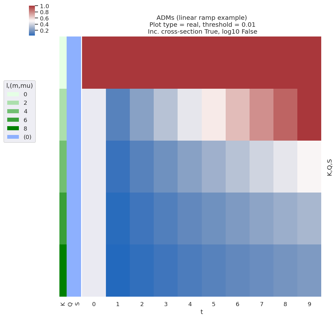
Fig. 3.7 Example ADMs used for AF basis function example (see Fig. 3.8). These ADMs essentially show an increasing degree of alignment with the \(t\) parameter, with high-order terms increasing at later \(t\).

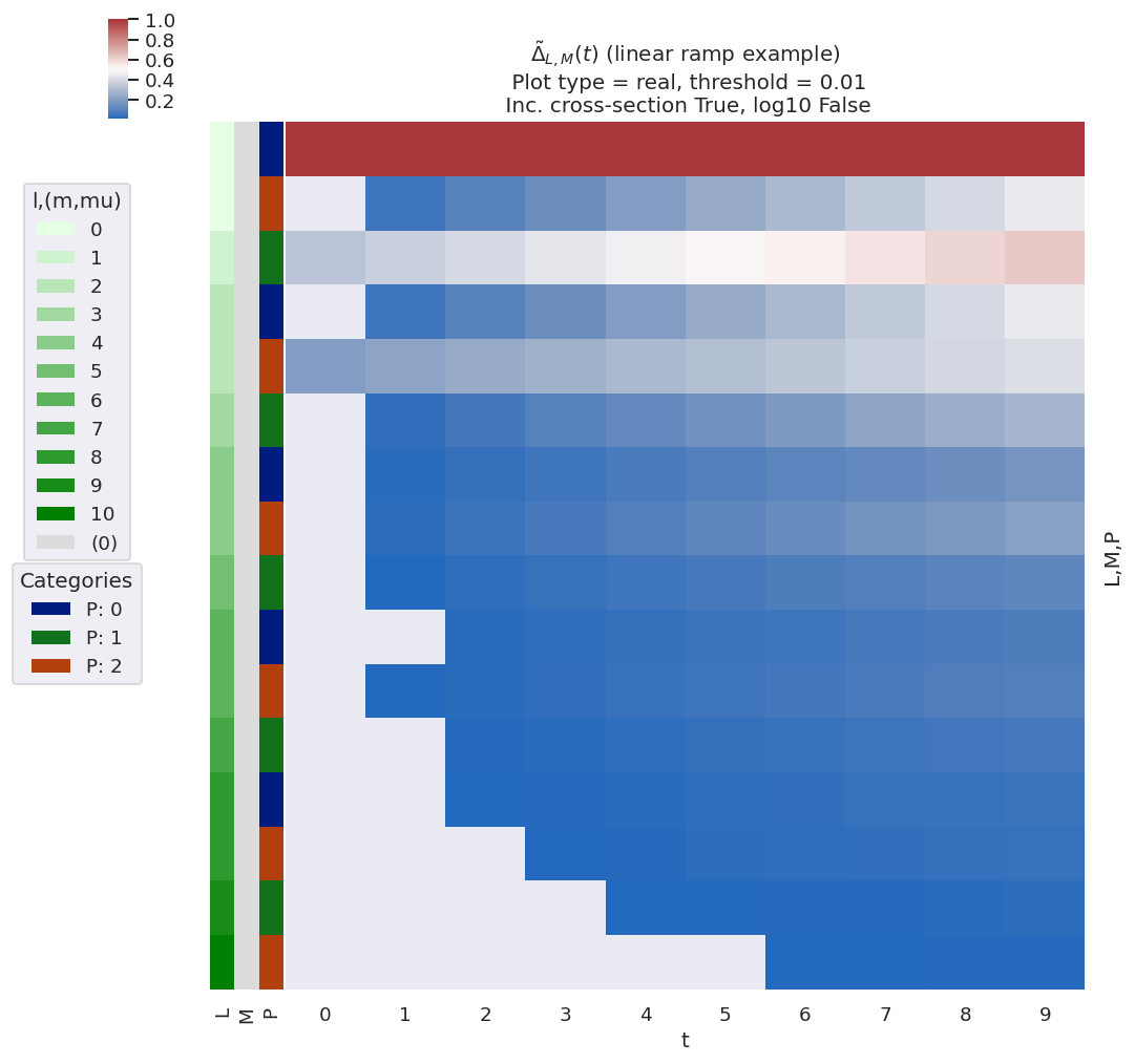
Fig. 3.8 Example of \(\tilde{\Delta}_{L,M}(t)\) basis values for various choices of alignment (as per Fig. 3.7). The ADMs essentially show an increasing degree of alignment with the \(t\) parameter, with high-order terms increasing at later \(t\), and this is reflected in the \(\tilde{\Delta}_{L,M}(t)\) terms with higher-order \(L\) appearing at later \(t\).

For cases with aligned molecular ensembles, additional terms can similarly appear depending on the alignment as well as the properties of the ionizing radiation. Again, the types of terms follow some typical patterns dependent on the symmetry of the ensemble, as well as the order of the terms allowed. For instance, \(L_{max}=P_{max}+K_{max}=2+K_{max}\), and \(K_{max}\) represents the overall degree of alignment of the ensemble; hence an aligned ensemble may be signified by higher-order terms in the observable (if allowed by other terms in the overall expansion) or, equivalently, aligning an ensemble prior to ionization can be used as a way to control which terms contribute to the alignment tensor.

Since this is a coherent averaging, additional interferences can also appear in the AF - or be restricted in the AF - depending on these geometric parameters and the contributing matrix elements. Additionally, any effects modulating these terms, for instance a time-dependent alignment (rotational wavepacket), vibronic dynamics (vibrational and/or electronic wavepacket), time-dependent laser field (control field) may be anticipated to lead to both changes in these terms and, potentially, interesting effects in the observable. Such effects have been discussed in more detail in Quantum Metrology Vol. 2 [9], and in the current case the focus is purely on rotational wavepackets.

Fig. 3.8 shows \(\tilde{\Delta}_{L,M}(t)\) for various choices of alignment (as per the ADMs shown in Fig. 3.7), and illustrates some of the general features discussed. Note, for example:

• \(L_{max}\) varies with alignment; in the demonstration case \(K_{max}=8\) at later times, resulting in \(L_{max}=10\), whilst at \(t=0\) \(K_{max}=0\), thus restricting terms to \(L_{max}=2\).

• Odd-\(L\) values are correlated with \(P=1\) terms.

• Only \(M=0\) terms are allowed in this case (\(Q=S=0\)).

3.3.8.2. 3D alignments and symmetry breaking

As discussed above, for the case where \(Q\neq0\) and/or \(S\neq0\) additional symmetry breaking can occur. It is simple to examine these effects numerically via changing the trial ADMs used to determine \(\tilde{\Delta}_{L,M}(t)\) (Eq. (3.28)), as illustrated in the following code block. (Realistic cases can be found in the case-studies presented in Part II.)

#*** Set range of ADMs for test as time-dependent values (linear ramps), 
#    including some trial "3D" alignment terms

# Set ADMs for increasing alignment...
# Here add some (arb) terms for Q,S non-zero (indexed as [K,Q,S, ADMs(t)])
tPoints = 10
inputADMs3D = [[0,0,0, *np.ones(tPoints)], 
             [2,0,0, *np.linspace(0,1,tPoints)], 
             [2,0,2, *np.linspace(0,0.5,tPoints)],
             [2,2,0, *np.linspace(0,0.5,tPoints)],
             [2,2,2, *np.linspace(0,0.8,tPoints)]]

# Set to AKQS parameters in an Xarray
AKQS = ep.setADMs(ADMs = inputADMs3D)

# Compute alignment terms
AFterm, DeltaTerm = ep.geomCalc.deltaLMKQS(EPR, AKQS)

#*** Plot subsection, L<=2, and sum over Rp and S-Rp terms
titleString = ('$\\tilde{\Delta}_{L,M}(t)$ (3D alignment ramp example).'
               '\n Summed over $R\'$ and $S-R\'$ terms.')
*_, gFig = ep.lmPlot(AFterm.where(AFterm.L<=2).sum('Rp').sum('S-Rp'),
                    xDim = 't', pType = 'r',
                    cmap='vlag',
                    titleString=titleString) 

# Glue versions for JupyterBook output
glue("ADMs-3DlinearRamp-lmPlot", gFig.fig, display=False)

Show code cell output Hide code cell output

Set dataType (No dataType)
Plotting data (No filename), pType=r, thres=0.01, with Seaborn

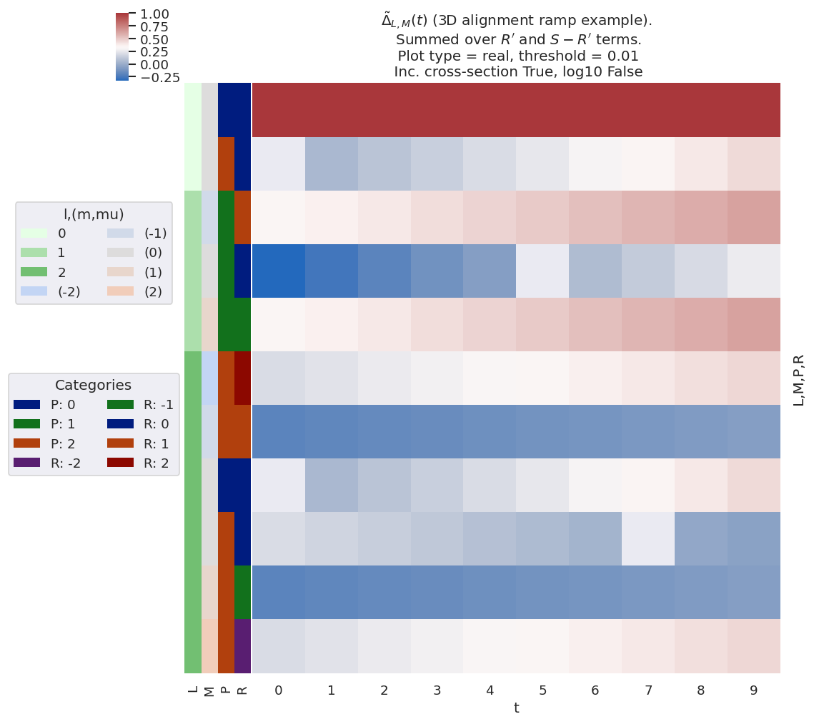
Fig. 3.9 Example \(\tilde{\Delta}_{L,M}(t)\) basis values for various choices of “3D” alignment, i.e. including some \(K\neq0\) and \(S\neq0\) terms. Note, in particular, the presence of \(M\neq0\) terms in general, and a complicated dependence of the allowed terms on the alignment (ADMs), which may increase, decrease, or even change sign for a given \(L,M\).

For illustration purposes, Fig. 3.9 shows a subselection of the \(\tilde{\Delta}_{L,M}(t)\) basis values, indicating some of the key features in the full 3D case, subselected for \(L\leq2\) and summed over \(R'\) and \(S-R'\) terms. Note, in particular, the presence of \(M\neq0\) terms in general, and a complicated dependence of the allowed terms on the alignment, which may increase, decrease, or even change sign. As previously, these behaviours are generally useful for understanding specific cases or planning experiments for specific systems; this is explored further in Part II which focuses on the results for particular molecules (hence symmetries and sets of matrix elements).

3.3.9. Tensor product terms

Following the above, further resultant terms can also be examined, up to and including the full channel functions \(\varUpsilon_{L,M}^{u,\zeta\zeta'}\) (see Eqn. (3.13)) for a given case. Numerically these are all implemented in the main ePSproc codebase [33, 34, 35], and can be returned by these functions for inspection - the full basis set already defined includes some of these products. Custom tensor product terms are also readily computed with the codebase, with tensor multiplications handled natively by the Xarray [53, 54] data objects (for more details of the data structures used, see the ePSproc documentation [35], specifically the data structures page).

The main product basis returned, labelled polProd in the output dictionary, contains the tensor product of the polarisation and alignment terms, \(\Lambda_{R}\otimes E_{PR}(\hat{e})\otimes \Delta_{L,M}(K,Q,S)\otimes A^{K}_{Q,S}(t)\), expanded over all quantum numbers (see full definition here). This term, therefore, incorporates all of the dependence (or response) of the AF-\(\beta_{LM}\)s on the polarisation state, and the axis distribution. Example results, making use of the linear-ramp ADMs of Sect. 3.3.8.1 are illustrated in Fig. 3.10.

The full channel (response) functions \(\varUpsilon_{L,M}^{u,\zeta\zeta'}\) as defined in (3.18) and (3.19) can be determined by the product of this term with the \(B_{L,M}\) tensor. This is essentially the complete geometric basis set, hence equivalent to the AF-\(\beta_{LM}\) if the ionization matrix elements were set to unity. This illustrates not only the coupling of the geometric terms into the observable \(L,M\), but also how the partial wave \(|l,m\rangle\) terms map to the observables, and hence the sensitivity of the observables to given partial wave properties. Example results, making use of the linear-ramp ADMs of Sect. 3.3.8.1 are illustrated in Fig. 3.11.

# Set data - set example ADMs to data structure & subset for calculation
data.setADMs(ADMs = inputADMs)
data.setSubset(dataKey = 'ADM', dataType = 'ADM')

# Using PEMtk - this only returns the product basis set as used for fitting
BetaNormX, basisProduct = data.afblmMatEfit(selDims={}, sqThres=False)

Subselected from dataset 'ADM', dataType 'ADM': 50 from 50 points (100.00%)

basisKey = 'polProd'  # Key for BLM basis set

# Plot with subselection on pol state (by label, 'A'=z-pol case)
titleString=('"Polprod" basis term, $\Lambda_{R}\otimes E_{PR}(\hat{e})\otimes' 
             '\Delta_{L,M}(K,Q,S)\otimes A^{K}_{Q,S}(t)$.'
             '\nSubselected for $z$-pol.')
*_, gFig = ep.lmPlot(basisProduct[basisKey].sel(Labels='A'), 
                   xDim='t', cmap = cmap, mDimLabel='mu',
                   labelCols=labelCols,
                   titleString=titleString);

# Glue versions for JupyterBook output
glue("polProd-linearRamp-lmPlot", gFig.fig, display=False)

Show code cell output Hide code cell output

Set dataType (No dataType)
Plotting data (No filename), pType=a, thres=0.01, with Seaborn

# Full channel functions
# Plot with subselection on pol state (by label, 'A'=z-pol case)
titleString='Channel functions example.\nSubselected for $z$-pol, $S-R\'=0$.'
*_, gFig =  ep.lmPlot((basisProduct['BLMtableResort'] * 
                       basisProduct['polProd']).sel(Labels='A').sel({'S-Rp':0}).sel(L=2), 
                      xDim='t', cmap=cmap, mDimLabel='m',
                      titleString=titleString); 

# Glue versions for JupyterBook output
glue("channelFunc-linearRamp-lmPlot", gFig.fig, display=False)

Show code cell output Hide code cell output

Set dataType (No dataType)
Plotting data (No filename), pType=a, thres=0.01, with Seaborn

No artists with labels found to put in legend.  Note that artists whose label start with an underscore are ignored when legend() is called with no argument.

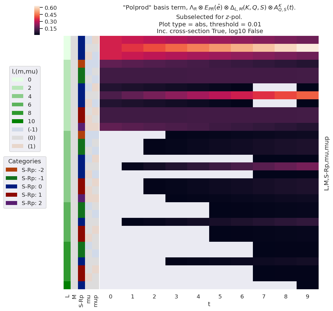
Fig. 3.10 Example product basis function for the polarisation and ADM terms, as given by \(\Lambda_{R}\otimes E_{PR}(\hat{e})\otimes \Delta_{L,M}(K,Q,S)\otimes A^{K}_{Q,S}(t)\). Shown for \(z\)-pol case only (\(p=0\)).

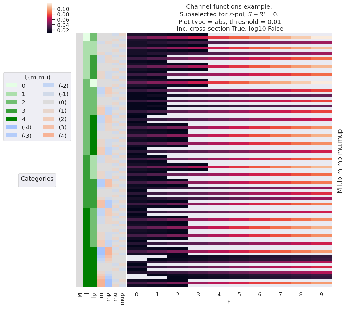
Fig. 3.11 Example of \(\bar{\varUpsilon_{}}_{L,M}^{u,\zeta\zeta'}\) basis values for various choices of alignment (as per Fig. 3.7), shown for \(L=2\) and \(z\)-pol case only (\(p=0\)). The basis essentially shows the obsevable terms if the ionization matrix elements are neglected, hence the sensitivity of the configuration to each pair of partial wave terms. Note, in general, that the sensitivity to any given pair \(\langle l',m'|l,m\rangle\), increases with alignment (hence with \(t\) in this example) for the linear polarisation case (\(\mu=\mu'=0\)), but typically decreases with alignment for cross-polarised terms.

---

[1]

Cf. the general form of Eq. (3.9). See also Quantum Metrology Vol. 2 [9] Chpt. 12 for early discussion and motivation for this formalism.