4. Numerical methodologies for extracting matrix elements#
Following the tensor notation outline in Sect. 3.3, the complete quantum metrology of a photoionization event (a.k.a. a “complete” photoionization experiment) can be characterized as recovery of the matrix elements \(I^{\zeta}(\epsilon)\) (per Eqs. (3.13), (3.14)) from the experimental measurements or, equivalently, the density matrix \(\mathbf{\rho}^{\zeta\zeta'}\) (Eqs. (3.31) - (3.33)). In general, such a recovery or reconstruction may be possible provided the channel functions are known, and the information content of the measurements is sufficient; it is, however, also possible that restrictions in any given case may preclude reconstruction, or restrict the level of recovery possible (e.g. to a lower symmetry group, or certain subsets of radial matrix elements) or fidelity of such a reconstruction. (For further discussion and background, see Refs. [92, 94] and Quantum Metrology Vol. 1 [4].)
Of particular import for radial matrix elements retrieval is the phase-sensitive nature of the observables (Sect. 3.6), which is required in order to obtain phase information on the partial-waves. In this context, PADs can also be considered as angular interferograms, and reconstruction can be considered conceptually similar to other phase-retrieval problems, e.g. optical field recovery with techniques such as FROG [127], and general quantum tomography [101].
As introduced previously (Sect. 1.1.2), the focus herein is the development and testing of the generalised bootstrap retrieval protocol, based on time-resolved RWP photoionization experiments. A general outline of the simplest 2-stage version of this protocol is shown in Fig. 4.1. In this scheme, the channel functions are assumed to be known, and the ADMs assumed to be accurately computable: these are, in general, required to determine the radial matrix elements in this protocol.
An extended outline comparing some similar approaches is shown in Fig. 4.2; of particular note here is the possibility for retrieval directly from MF measurements. Alternative, but conceptually similar, protocols involving different control parameters (as distinct from the RWP and MF cases), may also be also be used, see Quantum Metrology Vols. 1 & 2 [4, 9] for examples. For protocols making use of control methods, the key requirement is for the contribution of the control parameters to the observable, and associated coupling to the channel functions, to be accurately accounted for. In general, these contributions may be computed and/or obtained from experiment depending on the scheme used. One advantage of the RWP case is that the RWP can be accurately computed, and the determination of the corresponding molecular alignment (ADMs) from an experiment can be treated as a reduced-dimensionality linear signal retrieval problem. As indicated in Fig. 4.1, this stage is separable, and forms level 1 of the bootstrap retrieval protocol. In this procedure sets of computed ADMs form the basis set for the fitting (as a function of laser fluence and rotational temperature), allowing the accurate determination of the experimentally-achieved alignment; this is discussed further in Sect. 4.1.1. Level 2 involves non-linear data fitting, making use of the ADMs and the channel functions, in order to compute observables, and obtaining the radial matrix elements as the fitted parameters; this is discussed further in Sect. 4.1.2. [1]
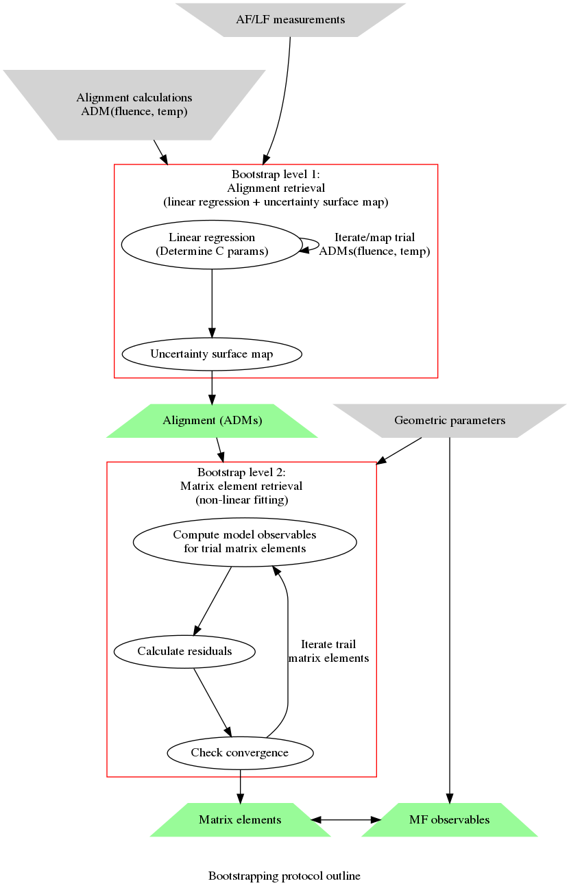
Fig. 4.1 Outline of the 2-stage generalised bootstrap radial matrix elements retrieval protocol (outlined conceptually in Sect. 1.1.2). In this case, level 1 outlines the determination of ADMs, and level 2 “bootstraps” from this to recover radial matrix elements and MF observables. Grey inverted trapezoids indicate required inputs to the protocol, green trapezoids indicate the retrieved quantities.#
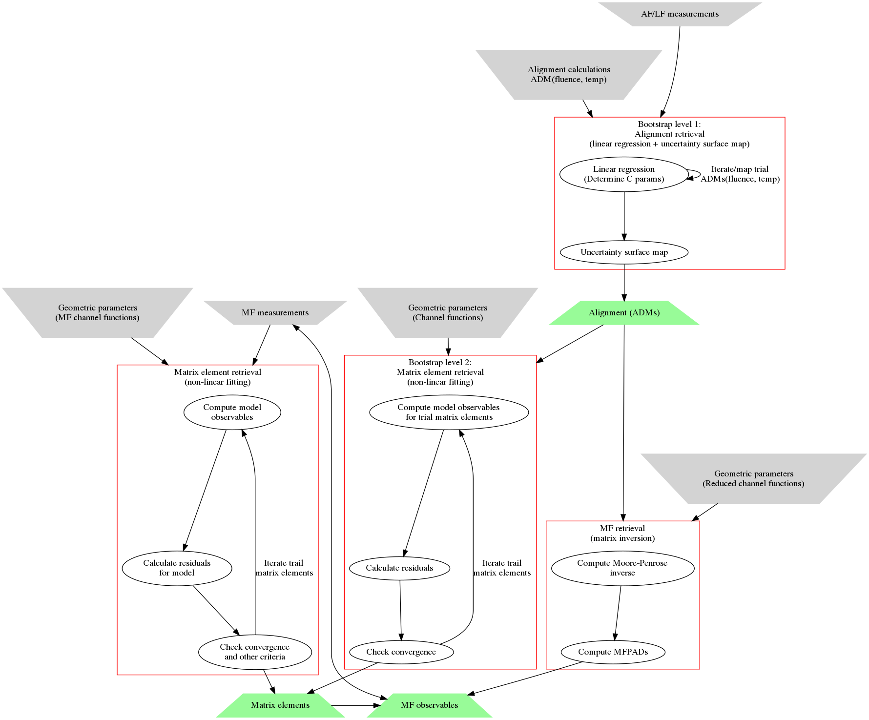
Fig. 4.2 Comparison of similar radial matrix elements retrieval protocols, illustrating (left) pure MF case; (middle) generalised bootstrap protocol; (lower right) matrix inversion protocol (see Ref. [98]); (top right) alignment retrieval. Grey inverted trapezoids indicate required inputs to the protocol, green trapezoids indicate the retrieved quantities. For the retrieval from the MF measurements case, no RWP and associated ADMs are required. For the matrix inversion protocol, MF observables are recovered, but not radial matrix elements, although the latter may be possible by subsequent analysis of the MF-PADs.#
4.1. Fitting methodologies#
In general, the extraction of parameters from a data set can be viewed as a general minimization (fitting) problem. This type of treatment is versatile, and can be multi-stage depending on the complexity of the problem. For the generalised bootstrapping method, the treatment of photoionization data is split into two types of fit, as shown in Fig. 4.1. Firstly, a linear fitting stage to retrieve the molecular axis distribution, characterised by a set of ADMs (see Sect. 3.3.8 for details); secondly, a non-linear fitting stage to retrieve the complex-valued matrix elements.
In terms of the data, the 1st stage can be written as:
And the 2nd stage as per Eqs. (3.13) and (3.17) for the AF case:
In these forms, the terms are:
\(A_{Q,S}^{K}(t)\), the set of ADMs defining the molecular alignment, and associated parameters \(\bar{C}_{KQS}^{LM}(\epsilon)\).
\(\bar{\varUpsilon_{}}_{L,M}^{u,\zeta\zeta'}(t)\), the channel functions in the AF (Eq. (3.17), and matrix elements \(\mathbb{I}^{\zeta\zeta'}(\epsilon)\).
Hence stage (2) relies on the inputs of stage (1), i.e. the ADMs; and the parameters in stage (1) can be determined via fitting the data (linear regression) making use of computed sets of \(A_{Q,S}^{K}(t)\) as a function of experimental parameters (laser fluence and rotational temperature). In this case, a range of ADMs (“basis sets”) are computed, and the best match to the experimental data chosen - more details are discussed in Sect. 4.1.1. In a similar manner, the 2nd stage makes use of a known basis set - the channel functions - but a non-linear fit is required to determine the set of matrix elements, see Sect. 4.1.2.
Finally, it is also of note that, although the case herein focusses on rotational wavepackets as a control parameter, the same general approach can be applied to other cases, e.g. fitting MF-PADs directly (for which only the 2nd stage is required), fitting PADs obtained via rotational state-resolved transitions, with shaped laser pulses and so on, as detailed in Quantum Metrology Vols. 1 & 2 [4, 9]. Although only rotational wavepacket cases are illustrated in this work (see Part II), by suitable choice of dataset and channel functions many other experimental schemes may be modelled and analysed; the Photoelectron Metrology Toolkit [5] is designed with this flexibility in mind.
4.1.1. Computation and linear fitting for alignment characterisation#
Efforts to align and orient molecules in recent decades have led to detailed studies of the rotational dynamics of molecules after interaction with a non-resonant femtosecond laser pulse. A significant outcome of these studies has been the development of a reliable model capable of accurate simulations of rotational wavepacket dynamics that quantitatively agree with experimental results. By measurement of a signal from a time evolving rotational wavepacket, this ability to accurately simulate the wavepacket dynamics can be used to reconstruct the measured signal in the MF. Since in this case the time resolved measurement constitutes a set of measurements of the same quantity from a variety of molecular axes distributions (sets of ADMs), it is reasonable to conclude that if the axes distributions are known, and provided a large enough space of orientations is explored by the molecule over the experimental time window, the MF signal should be extractable.
This is relatively straight forward for a signal that is a single number (scalar) in the MF for a given polarization of the light, such as the photoionization yield. Such a signal may, in general, be expressed as an expansion,
where \(\theta\) and \(\chi\) are the MF spherical polar and azimuthal angles of the linearly polarized electric field vector generating the signal (Sect. 3.3.3); \(C_{jk}\) are unknown expansion coefficients; and \(D^{j}_{0k}\) are the Wigner rotation matrix elements, a basis on the space of orientations. A time resolved measurement of \(S\) from a rotational wavepacket is the quantum expectation value of this expression,
Since the rotational wavepacket can be accurately simulated, the \(\langle D^{j}_{0k} \rangle (t)\) are considered known. From the measurement of a time resolved signal \(\langle S \rangle(t)\), the unknown coefficients \(C_{jk}\) can be determined by linear regression, and the molecular frame signal in Eq. (4.3) constructed. In this form the method was initially applied to strong field ionization and dubbed Orientation Reconstruction through Rotational Coherence Spectroscopy (ORRCS) [128, 129]. It has since been applied to strong field ionization of various molecules [130, 131, 132], strong field dissociation [133] and few-photon ionization [134].[2]
The case of PADs is a more challenging one, since they are not generally described by Eq. (4.3). Instead, both AF and MF-PADs are determined by the radial matrix elements, as discussed in Chpt. 3. However, the correspondence of the problem with an equation of the form of Eq. (4.4) - essentially a convolution - can be made. This is discussed in detail in Ref. [96]. In the current case Eqs. (3.13) and (3.17) can be rewritten in a similar form to Eq. (4.4) by explicitly separating out the ADMs \(A_{Q,S}^{K}(t)\) and collapsing all other terms. The case of photoionization from a time-dependent ensemble can then be reparameterized as indicated in Eq. (4.1). Here the set of axis distribution moments can thus be viewed as modulating all observables \(\beta_{L,M}^{u}(t)\). The unknowns, \(\bar{C}_{KQS}^{LM}\) and axis distribution moments \(A_{Q,S}^{K}(t)\), can be retrieved in a similar manner to that discussed for the simpler scalar observable case above (Eq. (4.4)), i.e. via linear regression with an RWP basis set.
In practice this equates to (accurately) simulating RWPs, hence obtaining the corresponding \(A_{Q,S}^{K}(t)\) parameters (expectation values), as a function of laser fluence and rotational temperature. Given experimental data, a 2D uncertainty (or error) surface in these two fundamental quantities can then be obtained from a linear regression for each set of \(A_{Q,S}^{K}(t)\). The closest set of parameters to the experimental case is then determined by selection of the best results (smallest uncertainty) from such a parameter-space mapping, which constitutes determination of both the rotational wavepacket (hence \(A_{Q,S}^{K}(t)\)) and \(\bar{C}_{KQS}^{LM}(\epsilon)\). Optimally, the corresponding physical properties can be cross-checked with other experimental estimates for additional confirmation of the fidelity of the protocol, although this may not always be possible. Note that, in this case, the photoionization dynamics are phenomenologically described by the real parameters \(\bar{C}_{KQS}^{LM}\), but details of the matrix elements are not obtained directly.
At the time of writing, computation of RWPs and this stage of the bootstrap retrieval protocol analysis is not implemented in the Photoelectron Metrology Toolkit [5], although is planned for the near future, and has been demonstrated in practice [1]. The examples in Part II instead make use of computed ADMs directly, essentially corresponding to the assumption that level 1 of the bootstrap retrieval protocol was successful. Given accurate RWPs, a successful fit to experimental data is generally assumed to be a given outcome, as this stage of the analysis requires only linear fitting in a two-parameter basis space.
4.1.2. Non-linear fitting for matrix elements#
The nature of the photoionization problem suggests that a fitting approach can work, in general, which can be expressed (for example) in the standard way as a (non-linear) least-squares minimization problem:
where \(\beta^{u}_{L,M}(\epsilon,t;\mathbb{I}^{\zeta\zeta'})\) denotes the values from a model function, computed for a given set of (complex) matrix elements \(\mathbb{I}^{\zeta\zeta'}\), and \(\beta^{u}_{L,M}(\epsilon,t)\) the experimentally-measured parameters, for a given configuration \(u\). Implicit in the notation is that the matrix elements are independent of \(u\) (or otherwise averaged over \(u\)). Once the matrix elements are obtained in this manner then MF observables, for any arbitrary \(u\), can be calculated. Generally fitting routines do not handle complex-valued functions, so the fitting parameter space is usually defined by parameters in magnitude-phase form (Eq. (3.15); see also discussion in Sect. 3.3.1)
Although in principle a very general approach, outstanding questions with such protocols remain, in particular fit uniqueness and reproducibility, the optimal measurement space \(u\) - or associated information content \(M_u\) - for any given case or measurement schema, how well they will scale to larger problems (more matrix elements/partial waves), the most efficient fitting methodologies/strategies, and so forth. In general, determination of radial matrix elements is not expected to be trivial, nor to always be successful, due to the complexity of the problem; one significant issue is the topology of the \(\chi^2\) hypersurface, which is of \(2N-1\) dimensions (where \(N\) is the number of radial matrix elements), and may contain local minima. Exploration of these questions for various exemplar systems is the topic of the Part II, and further general discussion can be found in Quantum Metrology Vols. 1 & 2 [4, 9], see in particular Quantum Metrology Vol. 2 [9] Sect. 8.2.2.
4.1.3. Implementation in PEMtk#
As outlined in Sect. 2.3 and Sect. 2.5, Photoelectron Metrology Toolkit [5] uses the lmfit library [66, 67] to implement general fitting routines, along with the ePSproc codebase [33, 34, 35] for computation of the required basis sets and observables. The latter has already been illustrated in Chpt. 3, and the illustration of the former is the subject of Part II. However, in these demonstrations only the RWP case is investigated, and analysis routines used only a standard Levenberg-Marquardt least-squares minimization method.
More generally, it is of note that the routines are written to be (somewhat) general and modular, such that other optimization methods may readily be implemented - either via those already supported by lmfit library [66, 67] (e.g. Levenberg-Marquardt, basinhopping, Nelder-Mead and so on - see the lmfit library [66, 67] documentation for supported methods), or by making use of other fitting libraries and methodologies.
Similarly, modification of the routines to other retrieval schemes should be fairly easy, and usually requires only:
a function which computes the required basis set (e.g. channel functions)
observables for the problem at hand.
Examples are given in Part II for the generalised bootstrap retrieval protocol, and MF-PADs based retrieval is also implemented in the codebase. For further details see the PEMtk documentation [20], particularly the fitting model backends and fitting MF and other datasets pages.
4.2. Fitting strategies#
The overall approach to complex non-linear fitting incorporates a number of aspects, broadly “fitting strategies”, which may influence the likelyhood of a successful radial matrix elements retrieval, and/or the time required to achieve this result:
The choice of numerical fitting method (Sect. 4.1.3).
The choice of dataset to analyse (and/or the choice of experimental measurement).
Additional statistical and/or other meta-analysis.
At the time of writing, work is ongoing in all these areas, and the illustrations in Part II herein include further notes regarding limitations or expectations for specific cases. Clearly, there are many choices numerically, and detailed investigation is required to determine the optimal strategy in any given case (this is examined partially in Part II in terms of limiting cases by symmetry). Emerging data analysis methods may also be useful here, in particular GPU-based routines and specialist high-dimensional space fitting methods.
One aspect that is intrinsic to these examples, but has not been discussed elsewhere, is the meta-analysis of the retrieved radial matrix elements. This is discussed generally in Quantum Metrology Vol. 2 [9] Sect. 8.2.2, and implemented numerically in the examples in Part II herein. The general aim in this type of analysis is to ascertain whether a given set of retrieved parameters is accurate and unique in a given case. Naturally, for test cases with synthetic data (as in Part II), testing against the known input radial matrix elements is the best solution and provides the most stringent test for the applicability of the retrieval method - but this is, of course, not generally useful for experimental datasets. Instead, as per previous analysis cases (see Quantum Metrology Vol. 2 [9]), a statistical (or “numerical experiment”) approach can be used. In this type of approach, a number of fits \(n\) (typically on the order of \(10^2\)-\(10^4\)) are run independently, with different seed parameters and/or different input data (cf. Monte Carlo methods, and statistical bootstrap methods), and the set of results analysed for consistency and uniqueness over the retrieved parameter sets. As outined in Quantum Metrology Vol. 2 [9] (updated to match the notation herein):
Each fit yields a solution set \(\mathbb{I}^{\zeta\zeta'}(n)\), with a final value of \(\chi^{2}(\mathbb{I}^{\zeta\zeta'}(n))\). Analysis of the fitted parameters \(\chi^{2}(\mathbb{I}^{\zeta\zeta'})\) can be employed to probe the behaviour of the fitting algorithm, and also to gain information on how well the experimental data defines each fitted parameter. Although it is non-trivial to visualize the full \(\chi^{2}\) hypersurface, aspects can be probed by plotting histograms and correlation plots of the fitted parameters. A large scatter in the value of a given fit parameter over a range of fits to the same data suggests a poorly defined parameter; a consistent result meanwhile shows that a particular parameter is well defined by the dataset. The experimental data can show different sensitivities to different parameters depending on the type of ionizing transitions present, because different transitions will (according to the magnitude of the geometrical parameters and symmetry constraints [i.e. channel functions herein]) be more sensitive to certain partial-waves. Additionally, the presence of multiple minima in the fit may be revealed by the presence of more than one feature in the histogram, reflecting more than one “best” fit result, while correlations appearing between supposedly uncorrelated parameters can indicate emergent behaviours in the high-dimensional space or - more prosaically - issues with the fitting methodology or coding.
—Quantum Metrology Vol. 2 [9], Chpt. 8
The same approach is taken in the case-studies of Part II, which include statistical analysis to determine the “correct” radial matrix elements from a set of non-linear fits, and associated uncertainties, again with the hope of illustrating general methods.