10. Case study: Generalised bootstrapping for a general asymmetric top scattering system, \(C_2H_4~(D_{2h})\)#
In this chapter, the full code and analysis details of the case study for \(C_2H_4\) are given, including obtaining required data, running fits and analysis routines. For more details on the routines, see the PEMtk documentation [20]; for the analysis see particularly the fit fidelity and analysis page, and molecular frame analysis data processing page (full analysis for Ref. [3], illustrating the \(N_2\) case).
10.1. General setup#
In the following code cells (see source notebooks for full details) the general setup routines (as per the outline in Chpt. 7 are executed via a configuration script with presets for the case studies herein.
Additionally, the routines will either run fits, or load existing data if available. Since fitting can be computationally demanding, it is, in general, recommended to approach large fitting problems carefully.
# Configure settings for case study
# Set case study by name
fitSystem='C2H4'
fitStem=f"fit_3D-test_withNoise_orb8"
# Add noise?
addNoise = 'y'
mu, sigma = 0, 0.05 # Up to approx 10% noise (+/- 0.05)
# Batching - number of fits to run between data dumps
batchSize = 10
# Total fits to run
nMax = 10
Show code cell content
# Run default config - may need to set full path here
%run '../scripts/setup_notebook_caseStudies_Mod-300723.py' # Test version with different figure options.
# %run '../scripts/setup_notebook.py'
# Set outputs for notebook or PDF (skips Holoviews plots unless glued)
# Note this is set to default 'pl' in script above
if buildEnv == 'pdf':
paramPlotBackend = 'sns' # For category plots with paramPlot
else:
paramPlotBackend = 'hv'
# plotBackend = 'sns' # For category plots with paramPlot
*** Setting up notebook with standard Quantum Metrology Vol. 3 imports...
For more details see https://pemtk.readthedocs.io/en/latest/fitting/PEMtk_fitting_basic_demo_030621-full.html
To use local source code, pass the parent path to this script at run time, e.g. "setup_fit_demo ~/github"
*** Running: 2023-12-07 10:48:39
Working dir: /home/jovyan/jake-home/buildTmp/_latest_build/html/doc-source/part2
Build env: html
None
* Loading packages...
* sparse not found, sparse matrix forms not available.
* natsort not found, some sorting functions not available.
* Setting plotter defaults with epsproc.basicPlotters.setPlotters(). Run directly to modify, or change options in local env.
* Set Holoviews with bokeh.
* pyevtk not found, VTK export not available.
* Set Holoviews with bokeh.
Jupyter Book : 0.15.1
External ToC : 0.3.1
MyST-Parser : 0.18.1
MyST-NB : 0.17.2
Sphinx Book Theme : 1.0.1
Jupyter-Cache : 0.6.1
NbClient : 0.7.4
# Pull data from web (C2H4 case)
from epsproc.util.io import getFilesFromGithub
# Set dataName (will be used as download subdir)
dataName = 'C2H4fitting'
# C2H4 matrix elements
GHbranch='3d-AFPAD-dev'
fDictMatE, fAllMatE = getFilesFromGithub(subpath='data/photoionization/C2H4', dataName=dataName, ref=GHbranch)
# C2H4 alignment data
fDictADM, fAllADM = getFilesFromGithub(subpath='data/alignment/C2H4_ADMs_8TW_120fs_VM', dataName=dataName, ref=GHbranch)
Querying URL: https://api.github.com/repos/phockett/epsproc/contents/data/photoionization/C2H4?ref=3d-AFPAD-dev
Local file /home/jovyan/jake-home/buildTmp/_latest_build/html/doc-source/part2/C2H4fitting/C2H4_1.0-100.0eV_orb8_B3u.inp.out already exists
Querying URL: https://api.github.com/repos/phockett/epsproc/contents/data/alignment/C2H4_ADMs_8TW_120fs_VM?ref=3d-AFPAD-dev
Local file /home/jovyan/jake-home/buildTmp/_latest_build/html/doc-source/part2/C2H4fitting/ADMs_8TW_120fs_5K.mat already exists
# Fitting setup including data generation and parameter creation
# Set datapath,
dataPath = Path(Path.cwd(),dataName)
ADMfile = 'ADMs_8TW_120fs_5K.mat'
# Run general config script with dataPath set above
%run "../scripts/setup_fit_case-studies_270723.py" -d {dataPath} -a {ADMfile} -c {fitSystem} -n {addNoise} --sigma {sigma}
Show code cell output
*** Setting up demo fitting workspace and main `data` class object...
Script: QM3 case studies
For more details see https://pemtk.readthedocs.io/en/latest/fitting/PEMtk_fitting_basic_demo_030621-full.html
To use local source code, pass the parent path to this script at run time, e.g. "setup_fit_demo ~/github"
* Loading packages...
* Loading demo matrix element data from /home/jovyan/jake-home/buildTmp/_latest_build/html/doc-source/part2/C2H4fitting
*** Job subset details
Key: subset
No 'job' info set for self.data[subset].
*** Job orb8 details
Key: orb8
Dir /home/jovyan/jake-home/buildTmp/_latest_build/html/doc-source/part2/C2H4fitting, 1 file(s).
{ 'batch': 'ePS ethylene, batch C2H4_1.0-100.0eV, orbital orb8_B3u',
'event': 'HOMO ioinzation (B3u), wavefn run, 0.5:1:10.5, sph grid',
'orbE': -10.32127880310325,
'orbLabel': 'B3u'}
* Loading demo ADM data from file /home/jovyan/jake-home/buildTmp/_latest_build/html/doc-source/part2/C2H4fitting/ADMs_8TW_120fs_5K.mat...
* Subselecting data...
Subselected from dataset 'orb8', dataType 'matE': 144 from 65520 points (0.22%)
Subselected from dataset 'pol', dataType 'pol': 1 from 3 points (33.33%)
Subselected from dataset 'ADM', dataType 'ADM': 1825 from 27575 points (6.62%)
* Calculating AF-BLMs...
Running for 73 t-points
Subselected from dataset 'sim', dataType 'AFBLM': 438 from 438 points (100.00%)
*Setting up fit parameters (with constraints)...
Set 38 complex matrix elements to 76 fitting params, see self.params for details.
Auto-setting parameters.
Basis set size = 76 params. Fitting with 14 magnitudes and 25 phases floated.
*** Adding Gaussian noise, mu=0, sigma=0.05
*** Setup demo fitting workspace OK.
Dataset: subset, AFBLM
Dataset: sim, AFBLM
| name | value | initial value | min | max | vary | expression |
|---|---|---|---|---|---|---|
| m_AG_B3U_B3U_0_0_n1_1 | 1.36649915 | 1.3664991519534047 | 1.0000e-04 | 5.00000000 | True | |
| m_AG_B3U_B3U_0_0_1_1 | 1.36649915 | 1.3664991519534047 | 1.0000e-04 | 5.00000000 | True | |
| m_AG_B3U_B3U_2_0_n1_1 | 1.29860947 | 1.2986094733813438 | 1.0000e-04 | 5.00000000 | True | |
| m_AG_B3U_B3U_2_0_1_1 | 1.29860947 | 1.2986094733813438 | 1.0000e-04 | 5.00000000 | True | |
| m_AG_B3U_B3U_2_n2_n1_1 | 1.38634203 | 1.3863420274695957 | 1.0000e-04 | 5.00000000 | True | |
| m_AG_B3U_B3U_2_n2_1_1 | 1.38634203 | 1.3863420274695957 | 1.0000e-04 | 5.00000000 | True | |
| m_AG_B3U_B3U_2_2_n1_1 | 1.38634203 | 1.3863420274695957 | 1.0000e-04 | 5.00000000 | False | m_AG_B3U_B3U_2_n2_n1_1 |
| m_AG_B3U_B3U_2_2_1_1 | 1.38634203 | 1.3863420274695957 | 1.0000e-04 | 5.00000000 | False | m_AG_B3U_B3U_2_n2_n1_1 |
| m_AG_B3U_B3U_4_0_n1_1 | 0.40035181 | 0.40035181362745503 | 1.0000e-04 | 5.00000000 | True | |
| m_AG_B3U_B3U_4_0_1_1 | 0.40035181 | 0.40035181362745503 | 1.0000e-04 | 5.00000000 | True | |
| m_AG_B3U_B3U_4_n2_n1_1 | 0.29998573 | 0.2999857331943446 | 1.0000e-04 | 5.00000000 | True | |
| m_AG_B3U_B3U_4_n2_1_1 | 0.29998573 | 0.2999857331943446 | 1.0000e-04 | 5.00000000 | True | |
| m_AG_B3U_B3U_4_2_n1_1 | 0.29998573 | 0.2999857331943446 | 1.0000e-04 | 5.00000000 | False | m_AG_B3U_B3U_4_n2_n1_1 |
| m_AG_B3U_B3U_4_2_1_1 | 0.29998573 | 0.2999857331943446 | 1.0000e-04 | 5.00000000 | False | m_AG_B3U_B3U_4_n2_n1_1 |
| m_AG_B3U_B3U_4_n4_n1_1 | 0.04982428 | 0.049824278378427615 | 1.0000e-04 | 5.00000000 | True | |
| m_AG_B3U_B3U_4_n4_1_1 | 0.04982428 | 0.049824278378427615 | 1.0000e-04 | 5.00000000 | True | |
| m_AG_B3U_B3U_4_4_n1_1 | 0.04982428 | 0.049824278378427615 | 1.0000e-04 | 5.00000000 | False | m_AG_B3U_B3U_4_n4_n1_1 |
| m_AG_B3U_B3U_4_4_1_1 | 0.04982428 | 0.049824278378427615 | 1.0000e-04 | 5.00000000 | False | m_AG_B3U_B3U_4_n4_n1_1 |
| m_AG_B3U_B3U_6_0_n1_1 | 0.01339645 | 0.013396454199331801 | 1.0000e-04 | 5.00000000 | True | |
| m_AG_B3U_B3U_6_0_1_1 | 0.01339645 | 0.013396454199331801 | 1.0000e-04 | 5.00000000 | True | |
| m_B1G_B3U_B2U_2_n2_n1_1 | 1.56318772 | 1.5631877150576254 | 1.0000e-04 | 5.00000000 | True | |
| m_B1G_B3U_B2U_2_n2_1_1 | 1.56318772 | 1.5631877150576254 | 1.0000e-04 | 5.00000000 | False | m_B1G_B3U_B2U_2_n2_n1_1 |
| m_B1G_B3U_B2U_2_2_n1_1 | 1.56318772 | 1.5631877150576254 | 1.0000e-04 | 5.00000000 | True | |
| m_B1G_B3U_B2U_2_2_1_1 | 1.56318772 | 1.5631877150576254 | 1.0000e-04 | 5.00000000 | False | m_B1G_B3U_B2U_2_n2_n1_1 |
| m_B1G_B3U_B2U_4_n2_n1_1 | 0.15371244 | 0.15371243514778368 | 1.0000e-04 | 5.00000000 | True | |
| m_B1G_B3U_B2U_4_n2_1_1 | 0.15371244 | 0.15371243514778368 | 1.0000e-04 | 5.00000000 | False | m_B1G_B3U_B2U_4_n2_n1_1 |
| m_B1G_B3U_B2U_4_2_n1_1 | 0.15371244 | 0.15371243514778368 | 1.0000e-04 | 5.00000000 | True | |
| m_B1G_B3U_B2U_4_2_1_1 | 0.15371244 | 0.15371243514778368 | 1.0000e-04 | 5.00000000 | False | m_B1G_B3U_B2U_4_n2_n1_1 |
| m_B1G_B3U_B2U_4_n4_n1_1 | 0.03535621 | 0.0353562103715001 | 1.0000e-04 | 5.00000000 | True | |
| m_B1G_B3U_B2U_4_n4_1_1 | 0.03535621 | 0.0353562103715001 | 1.0000e-04 | 5.00000000 | False | m_B1G_B3U_B2U_4_n4_n1_1 |
| m_B1G_B3U_B2U_4_4_n1_1 | 0.03535621 | 0.0353562103715001 | 1.0000e-04 | 5.00000000 | True | |
| m_B1G_B3U_B2U_4_4_1_1 | 0.03535621 | 0.0353562103715001 | 1.0000e-04 | 5.00000000 | False | m_B1G_B3U_B2U_4_n4_n1_1 |
| m_B2G_B3U_B1U_2_n1_0_1 | 0.52055662 | 0.5205566227796639 | 1.0000e-04 | 5.00000000 | True | |
| m_B2G_B3U_B1U_2_1_0_1 | 0.52055662 | 0.5205566227796639 | 1.0000e-04 | 5.00000000 | True | |
| m_B2G_B3U_B1U_4_n1_0_1 | 0.16248829 | 0.16248828678719807 | 1.0000e-04 | 5.00000000 | True | |
| m_B2G_B3U_B1U_4_1_0_1 | 0.16248829 | 0.16248828678719807 | 1.0000e-04 | 5.00000000 | True | |
| m_B2G_B3U_B1U_4_n3_0_1 | 0.07437621 | 0.07437621414570549 | 1.0000e-04 | 5.00000000 | True | |
| m_B2G_B3U_B1U_4_3_0_1 | 0.07437621 | 0.07437621414570549 | 1.0000e-04 | 5.00000000 | True | |
| p_AG_B3U_B3U_0_0_n1_1 | -2.97836575 | -2.978365751582027 | -3.14159265 | 3.14159265 | False | |
| p_AG_B3U_B3U_0_0_1_1 | 0.16322690 | 0.16322690200776627 | -3.14159265 | 3.14159265 | True | |
| p_AG_B3U_B3U_2_0_n1_1 | 0.75639421 | 0.7563942074737221 | -3.14159265 | 3.14159265 | True | |
| p_AG_B3U_B3U_2_0_1_1 | -2.38519845 | -2.385198446116071 | -3.14159265 | 3.14159265 | True | |
| p_AG_B3U_B3U_2_n2_n1_1 | -2.33986262 | -2.3398626225588375 | -3.14159265 | 3.14159265 | True | |
| p_AG_B3U_B3U_2_n2_1_1 | 0.80173003 | 0.8017300310309555 | -3.14159265 | 3.14159265 | True | |
| p_AG_B3U_B3U_2_2_n1_1 | -2.33986262 | -2.3398626225588375 | -3.14159265 | 3.14159265 | False | p_AG_B3U_B3U_2_n2_n1_1 |
| p_AG_B3U_B3U_2_2_1_1 | 0.80173003 | 0.8017300310309555 | -3.14159265 | 3.14159265 | False | p_AG_B3U_B3U_2_n2_1_1 |
| p_AG_B3U_B3U_4_0_n1_1 | -0.64744503 | -0.6474450252176692 | -3.14159265 | 3.14159265 | True | |
| p_AG_B3U_B3U_4_0_1_1 | 2.49414763 | 2.494147628372124 | -3.14159265 | 3.14159265 | True | |
| p_AG_B3U_B3U_4_n2_n1_1 | 0.21178197 | 0.2117819666136202 | -3.14159265 | 3.14159265 | True | |
| p_AG_B3U_B3U_4_n2_1_1 | -2.92981069 | -2.929810686976173 | -3.14159265 | 3.14159265 | True | |
| p_AG_B3U_B3U_4_2_n1_1 | 0.21178197 | 0.2117819666136202 | -3.14159265 | 3.14159265 | False | p_AG_B3U_B3U_4_n2_n1_1 |
| p_AG_B3U_B3U_4_2_1_1 | -2.92981069 | -2.929810686976173 | -3.14159265 | 3.14159265 | False | p_AG_B3U_B3U_4_n2_1_1 |
| p_AG_B3U_B3U_4_n4_n1_1 | 3.03975715 | 3.0397571534666024 | -3.14159265 | 3.14159265 | True | |
| p_AG_B3U_B3U_4_n4_1_1 | -0.10183550 | -0.10183550012319094 | -3.14159265 | 3.14159265 | True | |
| p_AG_B3U_B3U_4_4_n1_1 | 3.03975715 | 3.0397571534666024 | -3.14159265 | 3.14159265 | False | p_AG_B3U_B3U_4_n4_n1_1 |
| p_AG_B3U_B3U_4_4_1_1 | -0.10183550 | -0.10183550012319094 | -3.14159265 | 3.14159265 | False | p_AG_B3U_B3U_4_n4_1_1 |
| p_AG_B3U_B3U_6_0_n1_1 | 3.08008195 | 3.08008194969433 | -3.14159265 | 3.14159265 | True | |
| p_AG_B3U_B3U_6_0_1_1 | -0.06151070 | -0.06151070389546317 | -3.14159265 | 3.14159265 | True | |
| p_B1G_B3U_B2U_2_n2_n1_1 | 0.99264454 | 0.9926445369862835 | -3.14159265 | 3.14159265 | True | |
| p_B1G_B3U_B2U_2_n2_1_1 | 0.99264454 | 0.9926445369862835 | -3.14159265 | 3.14159265 | False | p_B1G_B3U_B2U_2_n2_n1_1 |
| p_B1G_B3U_B2U_2_2_n1_1 | -2.14894812 | -2.14894811660351 | -3.14159265 | 3.14159265 | True | |
| p_B1G_B3U_B2U_2_2_1_1 | -2.14894812 | -2.14894811660351 | -3.14159265 | 3.14159265 | False | p_B1G_B3U_B2U_2_2_n1_1 |
| p_B1G_B3U_B2U_4_n2_n1_1 | -2.02487007 | -2.024870073094406 | -3.14159265 | 3.14159265 | True | |
| p_B1G_B3U_B2U_4_n2_1_1 | -2.02487007 | -2.024870073094406 | -3.14159265 | 3.14159265 | False | p_B1G_B3U_B2U_4_n2_n1_1 |
| p_B1G_B3U_B2U_4_2_n1_1 | 1.11672258 | 1.1167225804953873 | -3.14159265 | 3.14159265 | True | |
| p_B1G_B3U_B2U_4_2_1_1 | 1.11672258 | 1.1167225804953873 | -3.14159265 | 3.14159265 | False | p_B1G_B3U_B2U_4_2_n1_1 |
| p_B1G_B3U_B2U_4_n4_n1_1 | 0.03720420 | 0.03720420026468335 | -3.14159265 | 3.14159265 | True | |
| p_B1G_B3U_B2U_4_n4_1_1 | 0.03720420 | 0.03720420026468335 | -3.14159265 | 3.14159265 | False | p_B1G_B3U_B2U_4_n4_n1_1 |
| p_B1G_B3U_B2U_4_4_n1_1 | -3.10438845 | -3.10438845332511 | -3.14159265 | 3.14159265 | True | |
| p_B1G_B3U_B2U_4_4_1_1 | -3.10438845 | -3.10438845332511 | -3.14159265 | 3.14159265 | False | p_B1G_B3U_B2U_4_4_n1_1 |
| p_B2G_B3U_B1U_2_n1_0_1 | 2.49526682 | 2.4952668185494518 | -3.14159265 | 3.14159265 | True | |
| p_B2G_B3U_B1U_2_1_0_1 | -0.64632584 | -0.6463258350403417 | -3.14159265 | 3.14159265 | True | |
| p_B2G_B3U_B1U_4_n1_0_1 | 2.06274363 | 2.0627436330964093 | -3.14159265 | 3.14159265 | True | |
| p_B2G_B3U_B1U_4_1_0_1 | -1.07884902 | -1.078849020493384 | -3.14159265 | 3.14159265 | True | |
| p_B2G_B3U_B1U_4_n3_0_1 | 1.97365959 | 1.9736595906190122 | -3.14159265 | 3.14159265 | True | |
| p_B2G_B3U_B1U_4_3_0_1 | -1.16793306 | -1.1679330629707811 | -3.14159265 | 3.14159265 | True |
10.2. Load existing fit data or run fits#
Note that running fits may be quite time-consuming and computationally intensive, depending on the size of the size of the problem. The default case here will run a small batch for testing if there is no existing data found on the dataPath, otherwise the data is loaded for analysis.
# Look for existing Pickle files on path
dataFiles = list(dataPath.expanduser().glob('*.pickle'))
if not dataFiles:
print("No data found, executing minimal fitting run...")
# Run fit batch - single
# data.multiFit(nRange = [n,n+batchSize-1], num_workers=batchSize)
# Run fit batches with checkpoint files
for n in np.arange(0,nMax,batchSize):
print(f'*** Running batch [{n},{n+batchSize-1}], {dt.now().strftime("%d%m%y_%H-%M-%S")}')
# Run fit batch
data.multiFit(nRange = [n,n+batchSize-1], num_workers=batchSize)
# Dump data so far
data.writeFitData(outStem=f"{fitSystem}_{n+batchSize-1}_{fitStem}")
print(f'Finished batch [{n},{n+batchSize-1}], {dt.now().strftime("%d%m%y_%H-%M-%S")}')
print(f'Written to file {fitSystem}_{n+batchSize-1}_{fitStem}')
else:
dataFileIn = dataFiles[-1] # Add index to select file, although loadFitData will concat multiple files
# Note that concat currently only works for fixed batch sizes however.
print(f"Set dataFiles: {dataFileIn}")
data.loadFitData(fList=dataFileIn, dataPath=dataPath) #.expanduser())
data.BLMfitPlot(keys=['subset','sim'])
# # Check ADMs
# data.data['subset']['ADM'].unstack().where(data.data['subset']['ADM'].unstack().K>0) \
# .real.hvplot.line(x='t').overlay(['K','Q','S'])
Set dataFiles: /home/jovyan/jake-home/buildTmp/_latest_build/html/doc-source/part2/C2H4fitting/C2H4_399_fit_3D-test_withNoise_orb8_270723_13-45-22.pickle
Read data from /home/jovyan/jake-home/buildTmp/_latest_build/html/doc-source/part2/C2H4fitting/C2H4_399_fit_3D-test_withNoise_orb8_270723_13-45-22.pickle with pickle.
Dataset: subset, AFBLM
Dataset: sim, AFBLM
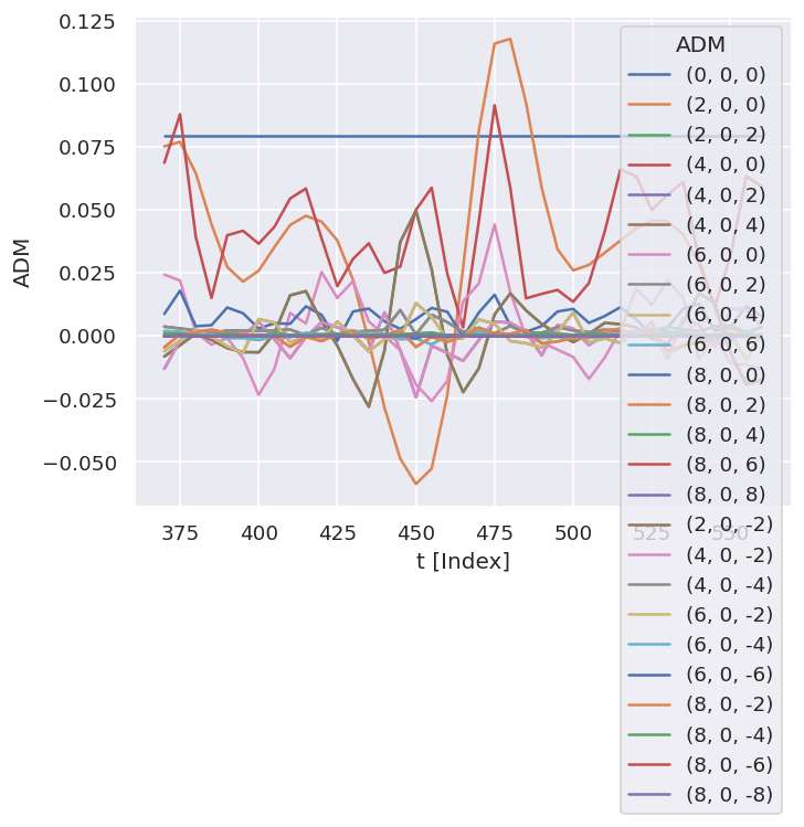
# Check ADMs
# Basic plotter
data.ADMplot(keys = 'subset')
Dataset: subset, ADM
Show code cell content
# Check ADMs
# Holoviews
data.data['subset']['ADM'].unstack().where(data.data['subset']['ADM'].unstack().K>0) \
.real.hvplot.line(x='t').overlay(['K','Q','S'])
# Fits appear as integer indexed items in the main data structure.
data.data.keys()
Show code cell output
dict_keys(['subset', 'orb8', 'ADM', 'pol', 'sim', 0, 1, 2, 3, 4, 5, 6, 7, 8, 9, 10, 11, 12, 13, 14, 15, 16, 17, 18, 19, 20, 21, 22, 23, 24, 25, 26, 27, 28, 29, 30, 31, 32, 33, 34, 35, 36, 37, 38, 40, 41, 42, 43, 44, 45, 46, 47, 48, 49, 50, 51, 52, 53, 54, 55, 56, 57, 58, 59, 60, 61, 62, 63, 64, 65, 66, 67, 68, 69, 70, 71, 72, 73, 74, 75, 76, 77, 78, 80, 81, 82, 83, 84, 85, 86, 87, 88, 89, 90, 91, 92, 93, 94, 95, 96, 97, 98, 99, 100, 101, 102, 103, 104, 105, 106, 107, 108, 109, 110, 111, 112, 113, 114, 115, 116, 117, 118, 120, 121, 122, 123, 124, 125, 126, 127, 128, 129, 130, 131, 132, 133, 134, 135, 136, 137, 138, 139, 140, 141, 142, 143, 144, 145, 146, 147, 148, 149, 150, 151, 152, 153, 154, 155, 156, 157, 158, 160, 161, 162, 163, 164, 165, 166, 167, 168, 169, 170, 171, 172, 173, 174, 175, 176, 177, 178, 179, 180, 181, 182, 183, 184, 185, 186, 187, 188, 189, 190, 191, 192, 193, 194, 195, 196, 197, 198, 200, 201, 202, 203, 204, 205, 206, 207, 208, 209, 210, 211, 212, 213, 214, 215, 216, 217, 218, 219, 220, 221, 222, 223, 224, 225, 226, 227, 228, 229, 230, 231, 232, 233, 234, 235, 236, 237, 238, 240, 241, 242, 243, 244, 245, 246, 247, 248, 249, 250, 251, 252, 253, 254, 255, 256, 257, 258, 259, 260, 261, 262, 263, 264, 265, 266, 267, 268, 269, 270, 271, 272, 273, 274, 275, 276, 277, 278, 280, 281, 282, 283, 284, 285, 286, 287, 288, 289, 290, 291, 292, 293, 294, 295, 296, 297, 298, 299, 300, 301, 302, 303, 304, 305, 306, 307, 308, 309, 310, 311, 312, 313, 314, 315, 316, 317, 318, 320, 321, 322, 323, 324, 325, 326, 327, 328, 329, 330, 331, 332, 333, 334, 335, 336, 337, 338, 339, 340, 341, 342, 343, 344, 345, 346, 347, 348, 349, 350, 351, 352, 353, 354, 355, 356, 357, 358, 360, 361, 362, 363, 364, 365, 366, 367, 368, 369, 370, 371, 372, 373, 374, 375, 376, 377, 378, 379, 380, 381, 382, 383, 384, 385, 386, 387, 388, 389, 390, 391, 392, 393, 394, 395, 396, 397, 398])
10.3. Post-processing and data overview#
Post-processing involves aggregation of all the fit run results into a single data structure. This can then be analysed statistically and examined for for best-fit results. In the statistical sense, this is essentailly a search for candidate radial matrix elements, based on the assumption that some of the minima found in the \(\chi^2\) hyperspace will be the true results. Even if a clear global minima does not exist, searching for candidate radial matrix elements sets based on clustering of results and multiple local minima is still expected to lead to viable candidates provided that the information content of the dataset is sufficient. However, as discussed elsewhere (see Sect. 4.2), in some cases this may not be the case, and other limitations may apply (e.g. certain parameters may be undefined), or additional data required for unique determination of the radial matrix elements.
For more details on the analysis routines, see the PEMtk documentation [20], particularly the fit fidelity and analysis page, and molecular frame analysis data processing page (full analysis for Ref. [3], illustrating the \(N_2\) case).
# General stats & post-processing to data tables
data.analyseFits()
*** Warning: found MultiIndex for DataFrame data.index - checkDims may have issues with Pandas MultiIndex, but will try anyway.
*** Warning: found MultiIndex for DataFrame data.index - checkDims may have issues with Pandas MultiIndex, but will try anyway.
{ 'Fits': 390,
'Minima': {'chisqr': 5.901473330378771e-05, 'redchi': 8.901166410827708e-08},
'Stats': { 'chisqr': min 5.901e-05
mean 2.760e-04
median 6.259e-05
max 3.133e-02
std 1.935e-03
var 3.746e-06
Name: chisqr, dtype: float64,
'redchi': min 8.901e-08
mean 4.164e-07
median 9.440e-08
max 4.726e-05
std 2.919e-06
var 8.521e-12
Name: redchi, dtype: float64},
'Success': 390}
# The BLMsetPlot routine will output aggregate fit results.
# Here the spread can be taken as a general indication of the uncertainty of
# the fitting, and indicate whether the fit is well-characterised/the information
# content of the data is sufficient.
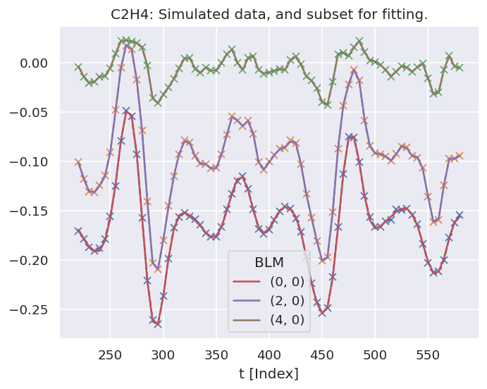
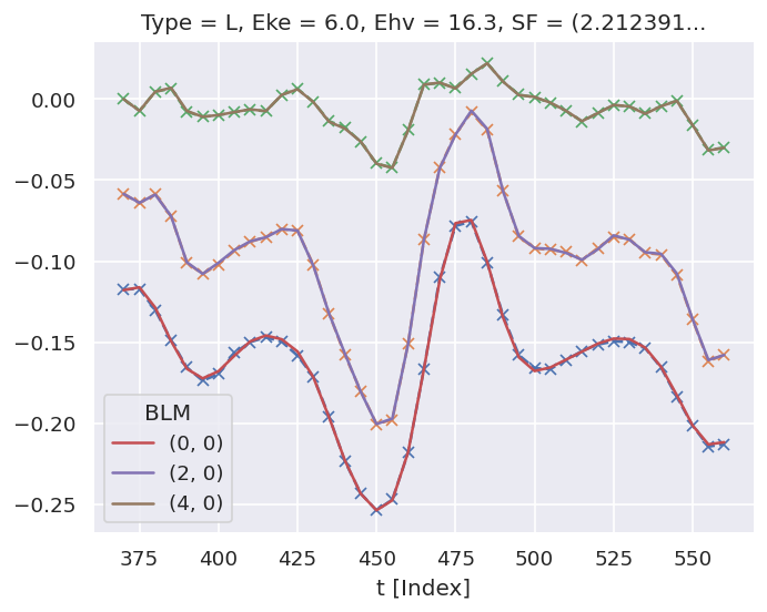
data.BLMsetPlot(xDim = 't', thres=1e-6) # With xDim and thres set, for more control over outputs
# Glue plot for later
glue("C2H4-fitResultsBLM",data.data['plots']['BLMsetPlot'])
Show code cell output
Fig. 10.1 Fit overview plot - \(\beta_{L,M}(t)\). Here dashed lines with ‘+’ markers indicates the input data, and bands indicate the mean fit results, where the width is the standard deviation in the fit model results. (See the PEMtk documentation [20] for details, particularly the analysis routines page.)#
# Write aggregate datasets to HDF5 format
# This is more robust than Pickled data, but PEMtk currently only support output for aggregate (post-processed) fit data.
data.processedToHDF5(dataPath = dataPath, outStem = dataFileIn.name, timeStamp=False)
Dumped self.data[fits][dfLong] to /home/jovyan/jake-home/buildTmp/_latest_build/html/doc-source/part2/C2H4fitting/C2H4_399_fit_3D-test_withNoise_orb8_270723_13-45-22.pickle_dfLong.pdHDF with Pandas .to_hdf() routine.
Dumped data to /home/jovyan/jake-home/buildTmp/_latest_build/html/doc-source/part2/C2H4fitting/C2H4_399_fit_3D-test_withNoise_orb8_270723_13-45-22.pickle_dfLong.pdHDF with pdHDF.
Dumped self.data[fits][AFxr] to /home/jovyan/jake-home/buildTmp/_latest_build/html/doc-source/part2/C2H4fitting/C2H4_399_fit_3D-test_withNoise_orb8_270723_13-45-22.pickle_AFxr.pdHDF with Pandas .to_hdf() routine.
Dumped data to /home/jovyan/jake-home/buildTmp/_latest_build/html/doc-source/part2/C2H4fitting/C2H4_399_fit_3D-test_withNoise_orb8_270723_13-45-22.pickle_AFxr.pdHDF with pdHDF.
# Histogram fit results (reduced chi^2 vs. fit index)
# This may be quite slow for large datasets, setting limited ranges may help
# Use default auto binning
# data.fitHist()
# Example with range set
data.fitHist(thres=3e-7, bins=100)
# Glue plot for later
glue("C2H4-fitHist",data.data['plots']['fitHistPlot'])
Mask selected 361 results (from 390).
Fig. 10.2 Fit overview plot - \(\chi^2\) vs. fit index. Here bands indicate groupings (local minima) are consistently found.#
Here, Fig. 10.1 shows an overview of the results compared with the input data, and Fig. 10.2 an overview of \(\chi^2\) vs. fit index. Bands in the \(\chi^2\) dimension can indicate groupings (local minima) are consistently found. Assuming each grouping is a viable fit candidate parameter set, these can then be explored in further detail.
10.4. Data exploration#
The general aim in this procedure is to ascertain whether there was a good spread of parameters explored, and a single (or few sets) of best-fit results. There are a few procedures and helper methods for this…
10.4.1. View results#
Single results sets can be viewed in the main data structure, indexed by integers.
# Check keys
fitNumber = 2
data.data[fitNumber].keys()
dict_keys(['AFBLM', 'residual', 'results'])
Here results is an lmFit object, which includes final fit results and information, and AFBLM contains the model (fit) output (i.e. resultant AF-\(\beta_{LM}\) values).
An example is shown below. Of particular note here is which parameters have vary=True - these are included in the fitting - and if there is a column expression, which indicates any parameters defined to have specific relationships (see Chpt. 6). Any correlations found during fitting are also shown, which can also indicate parameters which are related (even if this is not predefined or known a priori).
# Show some results
data.data[fitNumber]['results']
Show code cell output
Fit Result
| fitting method | leastsq |
| # function evals | 852 |
| # data points | 702 |
| # variables | 39 |
| chi-square | 1.3823e-04 |
| reduced chi-square | 2.0850e-07 |
| Akaike info crit. | -10761.2256 |
| Bayesian info crit. | -10583.6222 |
| name | value | standard error | relative error | initial value | min | max | vary | expression |
|---|---|---|---|---|---|---|---|---|
| m_AG_B3U_B3U_0_0_n1_1 | 1.51753751 | 1.6393e+08 | (10802655346.09%) | 0.8943598840733382 | 1.0000e-04 | 2.00000000 | True | |
| m_AG_B3U_B3U_0_0_1_1 | 1.51753751 | 1.6393e+08 | (10802655335.57%) | 0.8943598840733382 | 1.0000e-04 | 2.00000000 | False | m_AG_B3U_B3U_0_0_n1_1 |
| m_AG_B3U_B3U_2_0_n1_1 | 0.57410036 | 2.3095e+08 | (40228242220.61%) | 0.15487402637207892 | 1.0000e-04 | 2.00000000 | True | |
| m_AG_B3U_B3U_2_0_1_1 | 0.57410036 | 2.3095e+08 | (40228242090.86%) | 0.15487402637207892 | 1.0000e-04 | 2.00000000 | False | m_AG_B3U_B3U_2_0_n1_1 |
| m_AG_B3U_B3U_2_n2_n1_1 | 1.91353110 | 1.9621e+08 | (10253580188.91%) | 0.04122509840416122 | 1.0000e-04 | 2.00000000 | True | |
| m_AG_B3U_B3U_2_n2_1_1 | 1.91353110 | 1.9621e+08 | (10253580205.12%) | 0.04122509840416122 | 1.0000e-04 | 2.00000000 | False | m_AG_B3U_B3U_2_n2_n1_1 |
| m_AG_B3U_B3U_2_2_n1_1 | 1.91353110 | 1.9621e+08 | (10253580205.12%) | 0.04122509840416122 | 1.0000e-04 | 2.00000000 | False | m_AG_B3U_B3U_2_n2_n1_1 |
| m_AG_B3U_B3U_2_2_1_1 | 1.91353110 | 1.9621e+08 | (10253580205.12%) | 0.04122509840416122 | 1.0000e-04 | 2.00000000 | False | m_AG_B3U_B3U_2_n2_n1_1 |
| m_AG_B3U_B3U_4_0_n1_1 | 0.64063133 | 1.2293e+08 | (19189649770.62%) | 0.6607578301008963 | 1.0000e-04 | 2.00000000 | True | |
| m_AG_B3U_B3U_4_0_1_1 | 0.64063133 | 1.2293e+08 | (19189649783.48%) | 0.6607578301008963 | 1.0000e-04 | 2.00000000 | False | m_AG_B3U_B3U_4_0_n1_1 |
| m_AG_B3U_B3U_4_n2_n1_1 | 1.40792177 | 1.8641e+08 | (13240397601.64%) | 0.44813204588288 | 1.0000e-04 | 2.00000000 | True | |
| m_AG_B3U_B3U_4_n2_1_1 | 1.40792177 | 1.8641e+08 | (13240397595.45%) | 0.44813204588288 | 1.0000e-04 | 2.00000000 | False | m_AG_B3U_B3U_4_n2_n1_1 |
| m_AG_B3U_B3U_4_2_n1_1 | 1.40792177 | 1.8641e+08 | (13240397595.45%) | 0.44813204588288 | 1.0000e-04 | 2.00000000 | False | m_AG_B3U_B3U_4_n2_n1_1 |
| m_AG_B3U_B3U_4_2_1_1 | 1.40792177 | 1.8641e+08 | (13240397595.45%) | 0.44813204588288 | 1.0000e-04 | 2.00000000 | False | m_AG_B3U_B3U_4_n2_n1_1 |
| m_AG_B3U_B3U_4_n4_n1_1 | 1.44642889 | 24006024.2 | (1659675382.18%) | 0.6342937925832826 | 1.0000e-04 | 2.00000000 | True | |
| m_AG_B3U_B3U_4_n4_1_1 | 1.44642889 | 24006024.2 | (1659675380.80%) | 0.6342937925832826 | 1.0000e-04 | 2.00000000 | False | m_AG_B3U_B3U_4_n4_n1_1 |
| m_AG_B3U_B3U_4_4_n1_1 | 1.44642889 | 24006024.2 | (1659675380.80%) | 0.6342937925832826 | 1.0000e-04 | 2.00000000 | False | m_AG_B3U_B3U_4_n4_n1_1 |
| m_AG_B3U_B3U_4_4_1_1 | 1.44642889 | 24006024.2 | (1659675380.80%) | 0.6342937925832826 | 1.0000e-04 | 2.00000000 | False | m_AG_B3U_B3U_4_n4_n1_1 |
| m_AG_B3U_B3U_6_0_n1_1 | 1.0003e-04 | 17472.1784 | (17466813123.95%) | 0.8167122039927549 | 1.0000e-04 | 2.00000000 | True | |
| m_AG_B3U_B3U_6_0_1_1 | 1.0003e-04 | 17472.1784 | (17466813122.99%) | 0.8167122039927549 | 1.0000e-04 | 2.00000000 | False | m_AG_B3U_B3U_6_0_n1_1 |
| m_B1G_B3U_B2U_2_n2_n1_1 | 1.29634435 | 5.4415e+08 | (41975691314.28%) | 0.26802308590842283 | 1.0000e-04 | 2.00000000 | True | |
| m_B1G_B3U_B2U_2_n2_1_1 | 1.29634435 | 5.4415e+08 | (41975691202.81%) | 0.26802308590842283 | 1.0000e-04 | 2.00000000 | False | m_B1G_B3U_B2U_2_n2_n1_1 |
| m_B1G_B3U_B2U_2_2_n1_1 | 1.29634435 | 5.4415e+08 | (41975691202.81%) | 0.26802308590842283 | 1.0000e-04 | 2.00000000 | False | m_B1G_B3U_B2U_2_n2_n1_1 |
| m_B1G_B3U_B2U_2_2_1_1 | 1.29634435 | 5.4415e+08 | (41975691202.81%) | 0.26802308590842283 | 1.0000e-04 | 2.00000000 | False | m_B1G_B3U_B2U_2_n2_n1_1 |
| m_B1G_B3U_B2U_4_n2_n1_1 | 1.51498857 | 1.5428e+08 | (10183391854.62%) | 0.03957485857264054 | 1.0000e-04 | 2.00000000 | True | |
| m_B1G_B3U_B2U_4_n2_1_1 | 1.51498857 | 1.5428e+08 | (10183391833.96%) | 0.03957485857264054 | 1.0000e-04 | 2.00000000 | False | m_B1G_B3U_B2U_4_n2_n1_1 |
| m_B1G_B3U_B2U_4_2_n1_1 | 1.51498857 | 1.5428e+08 | (10183391833.96%) | 0.03957485857264054 | 1.0000e-04 | 2.00000000 | False | m_B1G_B3U_B2U_4_n2_n1_1 |
| m_B1G_B3U_B2U_4_2_1_1 | 1.51498857 | 1.5428e+08 | (10183391833.96%) | 0.03957485857264054 | 1.0000e-04 | 2.00000000 | False | m_B1G_B3U_B2U_4_n2_n1_1 |
| m_B1G_B3U_B2U_4_n4_n1_1 | 0.03590833 | 19150404.5 | (53331370872.86%) | 0.08480320665334273 | 1.0000e-04 | 2.00000000 | True | |
| m_B1G_B3U_B2U_4_n4_1_1 | 0.03590833 | 19150404.5 | (53331370859.56%) | 0.08480320665334273 | 1.0000e-04 | 2.00000000 | False | m_B1G_B3U_B2U_4_n4_n1_1 |
| m_B1G_B3U_B2U_4_4_n1_1 | 1.99999999 | 25993.4958 | (1299674.79%) | 0.5116101021743741 | 1.0000e-04 | 2.00000000 | True | |
| m_B1G_B3U_B2U_4_4_1_1 | 0.03590833 | 19150404.5 | (53331370859.56%) | 0.08480320665334273 | 1.0000e-04 | 2.00000000 | False | m_B1G_B3U_B2U_4_n4_n1_1 |
| m_B2G_B3U_B1U_2_n1_0_1 | 1.0023e-04 | 34307.4507 | (34228578961.99%) | 0.7225166884844292 | 1.0000e-04 | 2.00000000 | True | |
| m_B2G_B3U_B1U_2_1_0_1 | 1.0023e-04 | 34307.4507 | (34228578948.31%) | 0.7225166884844292 | 1.0000e-04 | 2.00000000 | False | m_B2G_B3U_B1U_2_n1_0_1 |
| m_B2G_B3U_B1U_4_n1_0_1 | 1.0002e-04 | 24770.7939 | (24764866247.09%) | 0.20555636227511953 | 1.0000e-04 | 2.00000000 | True | |
| m_B2G_B3U_B1U_4_1_0_1 | 1.0002e-04 | 24770.7939 | (24764866286.76%) | 0.20555636227511953 | 1.0000e-04 | 2.00000000 | False | m_B2G_B3U_B1U_4_n1_0_1 |
| m_B2G_B3U_B1U_4_n3_0_1 | 0.58378865 | 28400005.1 | (4864775159.92%) | 0.6939588949000473 | 1.0000e-04 | 2.00000000 | True | |
| m_B2G_B3U_B1U_4_3_0_1 | 0.58378865 | 28400005.1 | (4864775165.25%) | 0.6939588949000473 | 1.0000e-04 | 2.00000000 | False | m_B2G_B3U_B1U_4_n3_0_1 |
| p_AG_B3U_B3U_0_0_n1_1 | -2.97836575 | 0.00000000 | (0.00%) | -2.978365751582027 | -3.14159265 | 3.14159265 | False | |
| p_AG_B3U_B3U_0_0_1_1 | 3.14159264 | 276544.263 | (8802677.34%) | 0.2622639630066059 | -3.14159265 | 3.14159265 | True | |
| p_AG_B3U_B3U_2_0_n1_1 | 1.84335203 | 3.7512e+08 | (20350050824.75%) | 0.8321712969327423 | -3.14159265 | 3.14159265 | True | |
| p_AG_B3U_B3U_2_0_1_1 | -1.39167445 | 5.1820e+08 | (37236059352.06%) | 0.1667845863471027 | -3.14159265 | 3.14159265 | True | |
| p_AG_B3U_B3U_2_n2_n1_1 | 1.30317409 | 0.01081183 | (0.83%) | 0.8258955869067056 | -3.14159265 | 3.14159265 | True | |
| p_AG_B3U_B3U_2_n2_1_1 | -1.84459042 | 0.00288460 | (0.16%) | 0.5682807257100164 | -3.14159265 | 3.14159265 | True | |
| p_AG_B3U_B3U_2_2_n1_1 | 1.30317409 | 0.01081183 | (0.83%) | 0.8258955869067056 | -3.14159265 | 3.14159265 | False | p_AG_B3U_B3U_2_n2_n1_1 |
| p_AG_B3U_B3U_2_2_1_1 | -1.84459042 | 0.00288460 | (0.16%) | 0.5682807257100164 | -3.14159265 | 3.14159265 | False | p_AG_B3U_B3U_2_n2_1_1 |
| p_AG_B3U_B3U_4_0_n1_1 | -0.06969202 | 3.9944e+08 | (573146974460.17%) | 0.942523321466615 | -3.14159265 | 3.14159265 | True | |
| p_AG_B3U_B3U_4_0_1_1 | 3.11580277 | 6.5117e+08 | (20899060330.47%) | 0.4120221357980244 | -3.14159265 | 3.14159265 | True | |
| p_AG_B3U_B3U_4_n2_n1_1 | -1.80645487 | 0.23426057 | (12.97%) | 0.047931006169914414 | -3.14159265 | 3.14159265 | True | |
| p_AG_B3U_B3U_4_n2_1_1 | -0.12123851 | 0.00871302 | (7.19%) | 0.14528096836202342 | -3.14159265 | 3.14159265 | True | |
| p_AG_B3U_B3U_4_2_n1_1 | -1.80645487 | 0.23426057 | (12.97%) | 0.047931006169914414 | -3.14159265 | 3.14159265 | False | p_AG_B3U_B3U_4_n2_n1_1 |
| p_AG_B3U_B3U_4_2_1_1 | -0.12123851 | 0.00871302 | (7.19%) | 0.14528096836202342 | -3.14159265 | 3.14159265 | False | p_AG_B3U_B3U_4_n2_1_1 |
| p_AG_B3U_B3U_4_n4_n1_1 | 1.50273777 | 71560577.2 | (4762013617.80%) | 0.9861382375614064 | -3.14159265 | 3.14159265 | True | |
| p_AG_B3U_B3U_4_n4_1_1 | -1.98335989 | 1.1892e+08 | (5996050695.24%) | 0.5188969691954401 | -3.14159265 | 3.14159265 | True | |
| p_AG_B3U_B3U_4_4_n1_1 | 1.50273777 | 71560577.2 | (4762013614.94%) | 0.9861382375614064 | -3.14159265 | 3.14159265 | False | p_AG_B3U_B3U_4_n4_n1_1 |
| p_AG_B3U_B3U_4_4_1_1 | -1.98335989 | 1.1892e+08 | (5996050704.08%) | 0.5188969691954401 | -3.14159265 | 3.14159265 | False | p_AG_B3U_B3U_4_n4_1_1 |
| p_AG_B3U_B3U_6_0_n1_1 | -1.95314459 | 1.2267e+09 | (62807309790.12%) | 0.23657880041925605 | -3.14159265 | 3.14159265 | True | |
| p_AG_B3U_B3U_6_0_1_1 | -0.13873705 | 5.0431e+08 | (363502081206.21%) | 0.13243511128628982 | -3.14159265 | 3.14159265 | True | |
| p_B1G_B3U_B2U_2_n2_n1_1 | 2.77201773 | 7.0319e+08 | (25367334228.32%) | 0.24083316677882494 | -3.14159265 | 3.14159265 | True | |
| p_B1G_B3U_B2U_2_n2_1_1 | 2.77201773 | 7.0319e+08 | (25367334249.24%) | 0.24083316677882494 | -3.14159265 | 3.14159265 | False | p_B1G_B3U_B2U_2_n2_n1_1 |
| p_B1G_B3U_B2U_2_2_n1_1 | 2.15772653 | 3.0340e+08 | (14060977148.20%) | 0.913407849679565 | -3.14159265 | 3.14159265 | True | |
| p_B1G_B3U_B2U_2_2_1_1 | 2.15772653 | 3.0340e+08 | (14060977115.48%) | 0.913407849679565 | -3.14159265 | 3.14159265 | False | p_B1G_B3U_B2U_2_2_n1_1 |
| p_B1G_B3U_B2U_4_n2_n1_1 | 1.46179253 | 0.00972276 | (0.67%) | 0.5640600040603967 | -3.14159265 | 3.14159265 | True | |
| p_B1G_B3U_B2U_4_n2_1_1 | 1.46179253 | 0.00972276 | (0.67%) | 0.5640600040603967 | -3.14159265 | 3.14159265 | False | p_B1G_B3U_B2U_4_n2_n1_1 |
| p_B1G_B3U_B2U_4_2_n1_1 | -0.98792732 | 2.5715e+08 | (26029146287.96%) | 0.6627556088048271 | -3.14159265 | 3.14159265 | True | |
| p_B1G_B3U_B2U_4_2_1_1 | -0.98792732 | 2.5715e+08 | (26029146277.08%) | 0.6627556088048271 | -3.14159265 | 3.14159265 | False | p_B1G_B3U_B2U_4_2_n1_1 |
| p_B1G_B3U_B2U_4_n4_n1_1 | 3.12670378 | 5.3014e+08 | (16955308847.09%) | 0.5661233872989815 | -3.14159265 | 3.14159265 | True | |
| p_B1G_B3U_B2U_4_n4_1_1 | 3.12670378 | 5.3014e+08 | (16955308866.87%) | 0.5661233872989815 | -3.14159265 | 3.14159265 | False | p_B1G_B3U_B2U_4_n4_n1_1 |
| p_B1G_B3U_B2U_4_4_n1_1 | 1.66631806 | 1.2162e+09 | (72989706184.35%) | 0.801023706437469 | -3.14159265 | 3.14159265 | True | |
| p_B1G_B3U_B2U_4_4_1_1 | 1.66631806 | 1.2162e+09 | (72989706285.12%) | 0.801023706437469 | -3.14159265 | 3.14159265 | False | p_B1G_B3U_B2U_4_4_n1_1 |
| p_B2G_B3U_B1U_2_n1_0_1 | -0.66263297 | 1.1724e+09 | (176926450804.24%) | 0.5499735761521103 | -3.14159265 | 3.14159265 | True | |
| p_B2G_B3U_B1U_2_1_0_1 | 2.54252912 | 9.1632e+08 | (36039566933.76%) | 0.13891550441024236 | -3.14159265 | 3.14159265 | True | |
| p_B2G_B3U_B1U_4_n1_0_1 | -1.74459216 | 1.4116e+08 | (8091080639.49%) | 0.35793314176377866 | -3.14159265 | 3.14159265 | True | |
| p_B2G_B3U_B1U_4_1_0_1 | -3.13741264 | 1.4000e+08 | (4462344018.98%) | 0.9336159608271 | -3.14159265 | 3.14159265 | True | |
| p_B2G_B3U_B1U_4_n3_0_1 | 2.51110099 | 2.4425e+08 | (9726919204.41%) | 0.32664661542159223 | -3.14159265 | 3.14159265 | True | |
| p_B2G_B3U_B1U_4_3_0_1 | -0.19129208 | 2.3075e+08 | (120626839212.22%) | 0.5110822486361611 | -3.14159265 | 3.14159265 | True |
| Parameter1 | Parameter 2 | Correlation |
|---|---|---|
| p_AG_B3U_B3U_2_n2_n1_1 | p_B1G_B3U_B2U_4_n2_n1_1 | +0.9539 |
| m_AG_B3U_B3U_2_0_n1_1 | m_AG_B3U_B3U_4_0_n1_1 | +0.9031 |
| p_B1G_B3U_B2U_4_4_n1_1 | p_B2G_B3U_B1U_4_n3_0_1 | +0.8996 |
| m_AG_B3U_B3U_4_0_n1_1 | p_AG_B3U_B3U_2_0_1_1 | +0.8856 |
| m_AG_B3U_B3U_2_n2_n1_1 | m_B1G_B3U_B2U_2_n2_n1_1 | +0.8653 |
| m_AG_B3U_B3U_2_n2_n1_1 | p_B1G_B3U_B2U_2_n2_n1_1 | +0.8584 |
| p_B1G_B3U_B2U_4_4_n1_1 | p_B2G_B3U_B1U_4_3_0_1 | +0.8219 |
| m_B1G_B3U_B2U_4_n2_n1_1 | p_B1G_B3U_B2U_4_2_n1_1 | +0.8034 |
| p_B2G_B3U_B1U_4_n1_0_1 | p_B2G_B3U_B1U_4_1_0_1 | +0.7686 |
| m_AG_B3U_B3U_2_0_n1_1 | p_AG_B3U_B3U_2_0_1_1 | +0.7634 |
| p_AG_B3U_B3U_2_0_n1_1 | p_AG_B3U_B3U_2_0_1_1 | +0.7591 |
| m_AG_B3U_B3U_4_0_n1_1 | p_AG_B3U_B3U_2_0_n1_1 | +0.7177 |
| m_B1G_B3U_B2U_2_n2_n1_1 | p_B1G_B3U_B2U_2_n2_n1_1 | +0.6935 |
| m_AG_B3U_B3U_4_n2_n1_1 | p_B1G_B3U_B2U_4_2_n1_1 | -0.6652 |
| p_B2G_B3U_B1U_4_n3_0_1 | p_B2G_B3U_B1U_4_3_0_1 | +0.6210 |
| p_AG_B3U_B3U_2_0_n1_1 | p_B1G_B3U_B2U_4_2_n1_1 | +0.6208 |
| p_B1G_B3U_B2U_2_n2_n1_1 | p_B1G_B3U_B2U_2_2_n1_1 | +0.6140 |
| m_B2G_B3U_B1U_4_n3_0_1 | p_B2G_B3U_B1U_4_n1_0_1 | +0.5930 |
| m_AG_B3U_B3U_4_n2_n1_1 | m_B1G_B3U_B2U_4_n2_n1_1 | -0.5895 |
| m_B2G_B3U_B1U_2_n1_0_1 | p_B2G_B3U_B1U_2_1_0_1 | +0.5698 |
| m_AG_B3U_B3U_2_0_n1_1 | p_AG_B3U_B3U_2_0_n1_1 | +0.5565 |
| p_AG_B3U_B3U_6_0_n1_1 | p_AG_B3U_B3U_6_0_1_1 | -0.5526 |
| p_AG_B3U_B3U_4_0_n1_1 | p_AG_B3U_B3U_4_0_1_1 | -0.5398 |
| m_B1G_B3U_B2U_4_n2_n1_1 | p_B1G_B3U_B2U_4_4_n1_1 | +0.5285 |
| m_B1G_B3U_B2U_4_n2_n1_1 | p_B1G_B3U_B2U_2_n2_n1_1 | +0.5250 |
| m_AG_B3U_B3U_4_n2_n1_1 | p_AG_B3U_B3U_2_0_n1_1 | -0.5129 |
| m_AG_B3U_B3U_4_n2_n1_1 | p_AG_B3U_B3U_2_0_1_1 | -0.4962 |
| m_B1G_B3U_B2U_4_n2_n1_1 | p_B2G_B3U_B1U_4_3_0_1 | +0.4925 |
| p_B1G_B3U_B2U_2_n2_n1_1 | p_B1G_B3U_B2U_4_2_n1_1 | +0.4885 |
| m_B2G_B3U_B1U_4_n3_0_1 | p_B2G_B3U_B1U_4_n3_0_1 | -0.4883 |
| m_B1G_B3U_B2U_4_n2_n1_1 | p_AG_B3U_B3U_4_0_n1_1 | +0.4827 |
| m_AG_B3U_B3U_2_0_n1_1 | m_AG_B3U_B3U_2_n2_n1_1 | +0.4745 |
| m_B2G_B3U_B1U_2_n1_0_1 | p_B2G_B3U_B1U_2_n1_0_1 | -0.4728 |
| m_B2G_B3U_B1U_2_n1_0_1 | m_B2G_B3U_B1U_4_n1_0_1 | -0.4697 |
| p_AG_B3U_B3U_4_0_n1_1 | p_B1G_B3U_B2U_4_2_n1_1 | +0.4658 |
| m_B1G_B3U_B2U_4_n2_n1_1 | p_B2G_B3U_B1U_4_n3_0_1 | +0.4632 |
| m_AG_B3U_B3U_4_n2_n1_1 | p_AG_B3U_B3U_4_0_n1_1 | -0.4622 |
| p_B2G_B3U_B1U_4_n1_0_1 | p_B2G_B3U_B1U_4_n3_0_1 | -0.4620 |
| m_B1G_B3U_B2U_4_n4_n1_1 | p_AG_B3U_B3U_4_n2_1_1 | -0.4594 |
| p_AG_B3U_B3U_2_0_n1_1 | p_B2G_B3U_B1U_4_3_0_1 | +0.4396 |
| p_AG_B3U_B3U_4_0_1_1 | p_B1G_B3U_B2U_4_2_n1_1 | +0.4341 |
| m_AG_B3U_B3U_4_n2_n1_1 | m_B2G_B3U_B1U_4_n3_0_1 | -0.4325 |
| p_AG_B3U_B3U_2_0_n1_1 | p_AG_B3U_B3U_4_0_1_1 | +0.4282 |
| m_AG_B3U_B3U_2_0_n1_1 | m_B1G_B3U_B2U_2_n2_n1_1 | +0.4206 |
| m_AG_B3U_B3U_0_0_n1_1 | p_B1G_B3U_B2U_4_2_n1_1 | -0.4148 |
| p_B1G_B3U_B2U_2_n2_n1_1 | p_B1G_B3U_B2U_4_4_n1_1 | +0.4102 |
| m_AG_B3U_B3U_4_n2_n1_1 | p_B2G_B3U_B1U_4_n1_0_1 | -0.4066 |
| p_B1G_B3U_B2U_2_2_n1_1 | p_B1G_B3U_B2U_4_2_n1_1 | +0.4037 |
| m_AG_B3U_B3U_4_n2_n1_1 | p_AG_B3U_B3U_6_0_n1_1 | -0.3990 |
| m_AG_B3U_B3U_2_0_n1_1 | m_B1G_B3U_B2U_4_n2_n1_1 | -0.3953 |
| p_AG_B3U_B3U_4_0_n1_1 | p_AG_B3U_B3U_6_0_n1_1 | +0.3900 |
| m_AG_B3U_B3U_4_0_n1_1 | p_AG_B3U_B3U_4_0_n1_1 | -0.3897 |
| m_B2G_B3U_B1U_4_n3_0_1 | p_B2G_B3U_B1U_4_1_0_1 | +0.3886 |
| m_AG_B3U_B3U_4_n2_n1_1 | p_B2G_B3U_B1U_4_3_0_1 | -0.3873 |
| p_B2G_B3U_B1U_2_n1_0_1 | p_B2G_B3U_B1U_2_1_0_1 | +0.3868 |
| m_AG_B3U_B3U_2_n2_n1_1 | p_AG_B3U_B3U_2_0_n1_1 | +0.3833 |
| m_B2G_B3U_B1U_4_n3_0_1 | p_B2G_B3U_B1U_4_3_0_1 | +0.3808 |
| p_AG_B3U_B3U_4_n4_1_1 | p_B2G_B3U_B1U_4_n3_0_1 | +0.3786 |
| p_AG_B3U_B3U_2_n2_n1_1 | p_AG_B3U_B3U_4_n2_1_1 | +0.3720 |
| m_AG_B3U_B3U_0_0_n1_1 | p_AG_B3U_B3U_2_0_n1_1 | -0.3659 |
| m_B1G_B3U_B2U_4_n2_n1_1 | p_B1G_B3U_B2U_2_2_n1_1 | +0.3649 |
| m_B1G_B3U_B2U_4_n4_n1_1 | m_B2G_B3U_B1U_4_n3_0_1 | -0.3601 |
| m_AG_B3U_B3U_4_n4_n1_1 | m_B1G_B3U_B2U_4_4_n1_1 | -0.3557 |
| m_AG_B3U_B3U_4_n2_n1_1 | p_B2G_B3U_B1U_4_1_0_1 | -0.3536 |
| m_AG_B3U_B3U_2_0_n1_1 | p_AG_B3U_B3U_4_0_n1_1 | -0.3506 |
| m_AG_B3U_B3U_0_0_n1_1 | m_AG_B3U_B3U_2_0_n1_1 | +0.3489 |
| m_AG_B3U_B3U_6_0_n1_1 | p_AG_B3U_B3U_6_0_n1_1 | -0.3489 |
| m_AG_B3U_B3U_6_0_n1_1 | p_B2G_B3U_B1U_2_1_0_1 | -0.3427 |
| m_B2G_B3U_B1U_4_n1_0_1 | p_B2G_B3U_B1U_4_n3_0_1 | -0.3353 |
| m_B1G_B3U_B2U_4_n2_n1_1 | p_AG_B3U_B3U_4_0_1_1 | +0.3346 |
| m_AG_B3U_B3U_6_0_n1_1 | p_AG_B3U_B3U_6_0_1_1 | -0.3340 |
| m_B2G_B3U_B1U_4_n1_0_1 | p_AG_B3U_B3U_6_0_1_1 | +0.3336 |
| m_B2G_B3U_B1U_4_n3_0_1 | p_B1G_B3U_B2U_4_n4_n1_1 | -0.3327 |
| m_AG_B3U_B3U_4_0_n1_1 | m_B1G_B3U_B2U_4_n2_n1_1 | -0.3260 |
| p_AG_B3U_B3U_4_0_n1_1 | p_B2G_B3U_B1U_4_1_0_1 | +0.3193 |
| m_B1G_B3U_B2U_4_n2_n1_1 | p_AG_B3U_B3U_6_0_n1_1 | +0.3191 |
| m_AG_B3U_B3U_2_n2_n1_1 | p_B1G_B3U_B2U_4_4_n1_1 | +0.3148 |
| p_AG_B3U_B3U_2_0_n1_1 | p_B1G_B3U_B2U_2_n2_n1_1 | +0.3142 |
| p_AG_B3U_B3U_6_0_n1_1 | p_B1G_B3U_B2U_4_2_n1_1 | +0.3135 |
| m_AG_B3U_B3U_0_0_n1_1 | p_AG_B3U_B3U_4_0_1_1 | -0.3117 |
| m_AG_B3U_B3U_6_0_n1_1 | p_AG_B3U_B3U_2_n2_1_1 | -0.3069 |
| m_AG_B3U_B3U_0_0_n1_1 | m_AG_B3U_B3U_4_n4_n1_1 | +0.3040 |
| p_B1G_B3U_B2U_4_2_n1_1 | p_B2G_B3U_B1U_4_3_0_1 | +0.3017 |
| m_B2G_B3U_B1U_2_n1_0_1 | p_AG_B3U_B3U_4_0_1_1 | +0.2972 |
| p_AG_B3U_B3U_2_n2_1_1 | p_AG_B3U_B3U_4_n2_n1_1 | +0.2965 |
| m_AG_B3U_B3U_2_n2_n1_1 | p_B1G_B3U_B2U_4_2_n1_1 | +0.2959 |
| m_B1G_B3U_B2U_4_n4_n1_1 | p_B1G_B3U_B2U_4_n4_n1_1 | +0.2946 |
| m_AG_B3U_B3U_6_0_n1_1 | p_AG_B3U_B3U_4_0_n1_1 | +0.2921 |
| m_B1G_B3U_B2U_2_n2_n1_1 | m_B2G_B3U_B1U_4_n1_0_1 | +0.2908 |
| p_AG_B3U_B3U_2_0_1_1 | p_B2G_B3U_B1U_4_3_0_1 | +0.2903 |
| p_AG_B3U_B3U_4_n4_1_1 | p_B2G_B3U_B1U_4_n1_0_1 | -0.2896 |
| m_B2G_B3U_B1U_2_n1_0_1 | p_B2G_B3U_B1U_4_n1_0_1 | +0.2890 |
| p_AG_B3U_B3U_4_0_1_1 | p_B2G_B3U_B1U_4_3_0_1 | +0.2871 |
| m_B1G_B3U_B2U_2_n2_n1_1 | p_B2G_B3U_B1U_4_n3_0_1 | -0.2825 |
| m_AG_B3U_B3U_0_0_n1_1 | m_B1G_B3U_B2U_4_n2_n1_1 | -0.2818 |
| m_AG_B3U_B3U_0_0_n1_1 | p_B2G_B3U_B1U_4_n3_0_1 | -0.2797 |
| m_B2G_B3U_B1U_2_n1_0_1 | p_AG_B3U_B3U_6_0_n1_1 | +0.2794 |
| m_AG_B3U_B3U_2_n2_n1_1 | m_B1G_B3U_B2U_4_n2_n1_1 | +0.2794 |
| p_AG_B3U_B3U_4_n4_1_1 | p_B1G_B3U_B2U_4_4_n1_1 | +0.2760 |
| p_B2G_B3U_B1U_4_1_0_1 | p_B2G_B3U_B1U_4_n3_0_1 | -0.2757 |
| p_B1G_B3U_B2U_4_2_n1_1 | p_B2G_B3U_B1U_4_n1_0_1 | +0.2748 |
| p_AG_B3U_B3U_4_n4_n1_1 | p_AG_B3U_B3U_6_0_n1_1 | -0.2747 |
| m_B1G_B3U_B2U_2_n2_n1_1 | p_AG_B3U_B3U_2_0_n1_1 | +0.2734 |
| m_AG_B3U_B3U_4_n4_n1_1 | p_AG_B3U_B3U_2_0_n1_1 | -0.2717 |
| m_AG_B3U_B3U_0_0_n1_1 | p_AG_B3U_B3U_0_0_1_1 | +0.2698 |
| m_B2G_B3U_B1U_4_n1_0_1 | p_AG_B3U_B3U_4_n4_1_1 | -0.2683 |
| m_B1G_B3U_B2U_4_n4_n1_1 | p_B2G_B3U_B1U_4_n3_0_1 | +0.2673 |
| m_B2G_B3U_B1U_4_n1_0_1 | p_B1G_B3U_B2U_4_4_n1_1 | -0.2637 |
| p_AG_B3U_B3U_6_0_n1_1 | p_B2G_B3U_B1U_4_n1_0_1 | +0.2629 |
| m_AG_B3U_B3U_0_0_n1_1 | p_B2G_B3U_B1U_4_3_0_1 | -0.2629 |
| m_B1G_B3U_B2U_4_n2_n1_1 | p_AG_B3U_B3U_2_0_n1_1 | +0.2619 |
| p_AG_B3U_B3U_2_0_1_1 | p_B1G_B3U_B2U_4_2_n1_1 | +0.2605 |
| m_B2G_B3U_B1U_4_n1_0_1 | m_B2G_B3U_B1U_4_n3_0_1 | +0.2597 |
| p_AG_B3U_B3U_4_n2_n1_1 | p_AG_B3U_B3U_4_n4_1_1 | +0.2589 |
| m_AG_B3U_B3U_0_0_n1_1 | p_AG_B3U_B3U_2_0_1_1 | +0.2551 |
| m_B1G_B3U_B2U_4_4_n1_1 | p_B2G_B3U_B1U_2_n1_0_1 | -0.2530 |
| m_B1G_B3U_B2U_2_n2_n1_1 | p_AG_B3U_B3U_4_n4_1_1 | -0.2506 |
| p_B1G_B3U_B2U_2_n2_n1_1 | p_B2G_B3U_B1U_4_3_0_1 | +0.2490 |
| m_AG_B3U_B3U_6_0_n1_1 | p_B2G_B3U_B1U_4_1_0_1 | +0.2470 |
| m_AG_B3U_B3U_4_n2_n1_1 | p_AG_B3U_B3U_4_n2_n1_1 | +0.2464 |
| p_AG_B3U_B3U_2_n2_1_1 | p_AG_B3U_B3U_6_0_n1_1 | +0.2449 |
| p_B1G_B3U_B2U_4_4_n1_1 | p_B2G_B3U_B1U_4_n1_0_1 | -0.2435 |
| m_B1G_B3U_B2U_4_n4_n1_1 | p_AG_B3U_B3U_4_n4_n1_1 | -0.2433 |
| p_AG_B3U_B3U_6_0_n1_1 | p_B1G_B3U_B2U_2_2_n1_1 | +0.2426 |
| m_AG_B3U_B3U_6_0_n1_1 | m_B2G_B3U_B1U_2_n1_0_1 | -0.2418 |
| p_AG_B3U_B3U_4_n4_n1_1 | p_B2G_B3U_B1U_4_n3_0_1 | +0.2413 |
| m_B1G_B3U_B2U_4_n4_n1_1 | p_B1G_B3U_B2U_4_4_n1_1 | +0.2405 |
| m_B2G_B3U_B1U_4_n3_0_1 | p_AG_B3U_B3U_2_0_n1_1 | +0.2401 |
| p_AG_B3U_B3U_4_n4_1_1 | p_B1G_B3U_B2U_2_2_n1_1 | +0.2393 |
| p_AG_B3U_B3U_2_0_n1_1 | p_B1G_B3U_B2U_4_4_n1_1 | +0.2392 |
| p_AG_B3U_B3U_0_0_1_1 | p_AG_B3U_B3U_4_n2_n1_1 | -0.2387 |
| p_AG_B3U_B3U_6_0_1_1 | p_B1G_B3U_B2U_4_4_n1_1 | -0.2370 |
| m_AG_B3U_B3U_4_n4_n1_1 | p_AG_B3U_B3U_4_0_1_1 | -0.2364 |
| m_AG_B3U_B3U_4_n4_n1_1 | p_B1G_B3U_B2U_4_2_n1_1 | -0.2350 |
| m_AG_B3U_B3U_0_0_n1_1 | p_AG_B3U_B3U_2_n2_1_1 | +0.2335 |
| p_AG_B3U_B3U_4_0_n1_1 | p_B2G_B3U_B1U_4_n1_0_1 | +0.2333 |
| m_B2G_B3U_B1U_4_n3_0_1 | p_AG_B3U_B3U_4_n4_1_1 | -0.2330 |
| p_AG_B3U_B3U_2_0_1_1 | p_AG_B3U_B3U_4_0_1_1 | +0.2323 |
| p_AG_B3U_B3U_2_0_1_1 | p_AG_B3U_B3U_2_n2_1_1 | +0.2322 |
| p_B1G_B3U_B2U_2_2_n1_1 | p_B2G_B3U_B1U_2_1_0_1 | +0.2315 |
| m_B1G_B3U_B2U_4_4_n1_1 | p_AG_B3U_B3U_4_0_1_1 | +0.2304 |
| m_B1G_B3U_B2U_2_n2_n1_1 | p_B1G_B3U_B2U_4_2_n1_1 | +0.2284 |
| p_AG_B3U_B3U_4_n2_n1_1 | p_B2G_B3U_B1U_4_n1_0_1 | -0.2277 |
| m_AG_B3U_B3U_2_0_n1_1 | p_AG_B3U_B3U_4_n4_1_1 | -0.2274 |
| m_AG_B3U_B3U_4_n2_n1_1 | p_AG_B3U_B3U_4_n4_1_1 | +0.2274 |
| m_AG_B3U_B3U_4_0_n1_1 | p_B2G_B3U_B1U_4_3_0_1 | +0.2264 |
| m_AG_B3U_B3U_0_0_n1_1 | p_B2G_B3U_B1U_2_1_0_1 | +0.2258 |
| p_B2G_B3U_B1U_2_1_0_1 | p_B2G_B3U_B1U_4_n1_0_1 | +0.2257 |
| p_B2G_B3U_B1U_2_1_0_1 | p_B2G_B3U_B1U_4_n3_0_1 | -0.2253 |
| m_AG_B3U_B3U_6_0_n1_1 | p_AG_B3U_B3U_4_0_1_1 | -0.2226 |
| m_AG_B3U_B3U_2_0_n1_1 | p_AG_B3U_B3U_2_n2_1_1 | +0.2221 |
| p_B1G_B3U_B2U_4_2_n1_1 | p_B2G_B3U_B1U_4_1_0_1 | +0.2210 |
| p_AG_B3U_B3U_0_0_1_1 | p_B1G_B3U_B2U_2_2_n1_1 | +0.2188 |
| m_B1G_B3U_B2U_4_n2_n1_1 | m_B1G_B3U_B2U_4_4_n1_1 | +0.2159 |
| p_AG_B3U_B3U_4_n2_n1_1 | p_B2G_B3U_B1U_4_1_0_1 | -0.2156 |
| m_AG_B3U_B3U_2_n2_n1_1 | p_B2G_B3U_B1U_4_3_0_1 | +0.2155 |
| p_AG_B3U_B3U_2_0_n1_1 | p_B2G_B3U_B1U_4_n3_0_1 | +0.2113 |
| m_B1G_B3U_B2U_4_n4_n1_1 | p_B2G_B3U_B1U_2_n1_0_1 | -0.2111 |
| p_B1G_B3U_B2U_4_n4_n1_1 | p_B2G_B3U_B1U_4_1_0_1 | -0.2104 |
| m_B2G_B3U_B1U_2_n1_0_1 | p_AG_B3U_B3U_6_0_1_1 | -0.2097 |
| m_B1G_B3U_B2U_4_n4_n1_1 | p_B1G_B3U_B2U_2_2_n1_1 | +0.2091 |
| m_AG_B3U_B3U_6_0_n1_1 | p_AG_B3U_B3U_4_n4_n1_1 | +0.2091 |
| p_AG_B3U_B3U_4_n2_1_1 | p_B1G_B3U_B2U_4_n4_n1_1 | -0.2090 |
| m_AG_B3U_B3U_2_n2_n1_1 | p_AG_B3U_B3U_4_n4_1_1 | -0.2088 |
| m_B1G_B3U_B2U_4_n4_n1_1 | p_AG_B3U_B3U_6_0_n1_1 | +0.2081 |
| m_AG_B3U_B3U_2_n2_n1_1 | m_AG_B3U_B3U_4_0_n1_1 | +0.2068 |
| m_AG_B3U_B3U_4_n4_n1_1 | p_B2G_B3U_B1U_4_3_0_1 | -0.2068 |
| m_B2G_B3U_B1U_4_n3_0_1 | p_B1G_B3U_B2U_4_2_n1_1 | +0.2062 |
| p_AG_B3U_B3U_4_n4_1_1 | p_B2G_B3U_B1U_4_1_0_1 | -0.2056 |
| p_AG_B3U_B3U_6_0_1_1 | p_B2G_B3U_B1U_4_n3_0_1 | -0.2055 |
| p_AG_B3U_B3U_4_n2_n1_1 | p_B1G_B3U_B2U_2_2_n1_1 | +0.2052 |
| m_AG_B3U_B3U_2_0_n1_1 | p_B1G_B3U_B2U_2_n2_n1_1 | +0.2050 |
| m_B1G_B3U_B2U_2_n2_n1_1 | m_B1G_B3U_B2U_4_4_n1_1 | -0.2044 |
| p_B1G_B3U_B2U_4_n4_n1_1 | p_B2G_B3U_B1U_4_n1_0_1 | -0.2038 |
| m_B1G_B3U_B2U_4_n2_n1_1 | p_AG_B3U_B3U_4_n4_1_1 | +0.2036 |
| m_B1G_B3U_B2U_4_4_n1_1 | p_B2G_B3U_B1U_4_n1_0_1 | +0.2025 |
| m_B1G_B3U_B2U_4_4_n1_1 | p_AG_B3U_B3U_4_n2_1_1 | +0.2006 |
| m_B1G_B3U_B2U_2_n2_n1_1 | p_B2G_B3U_B1U_4_3_0_1 | -0.2002 |
| p_B2G_B3U_B1U_2_n1_0_1 | p_B2G_B3U_B1U_4_n1_0_1 | -0.2000 |
| m_AG_B3U_B3U_6_0_n1_1 | p_B1G_B3U_B2U_4_n4_n1_1 | -0.1992 |
| m_B2G_B3U_B1U_4_n3_0_1 | p_B2G_B3U_B1U_2_1_0_1 | +0.1989 |
| p_AG_B3U_B3U_4_n2_1_1 | p_AG_B3U_B3U_4_n4_1_1 | +0.1980 |
| m_AG_B3U_B3U_4_n2_n1_1 | p_AG_B3U_B3U_4_0_1_1 | -0.1960 |
| p_AG_B3U_B3U_4_n4_1_1 | p_B1G_B3U_B2U_4_2_n1_1 | +0.1956 |
| p_AG_B3U_B3U_4_n2_1_1 | p_B1G_B3U_B2U_4_n2_n1_1 | +0.1947 |
| m_B1G_B3U_B2U_4_4_n1_1 | p_B2G_B3U_B1U_4_3_0_1 | +0.1944 |
| m_AG_B3U_B3U_2_0_n1_1 | p_B2G_B3U_B1U_2_n1_0_1 | +0.1935 |
| m_AG_B3U_B3U_0_0_n1_1 | p_B1G_B3U_B2U_4_n4_n1_1 | -0.1934 |
| m_B1G_B3U_B2U_2_n2_n1_1 | p_B2G_B3U_B1U_4_n1_0_1 | +0.1925 |
| p_AG_B3U_B3U_2_n2_1_1 | p_AG_B3U_B3U_4_0_n1_1 | -0.1924 |
| p_AG_B3U_B3U_4_n4_1_1 | p_B2G_B3U_B1U_4_3_0_1 | +0.1919 |
| p_AG_B3U_B3U_2_0_1_1 | p_B2G_B3U_B1U_2_1_0_1 | +0.1910 |
| p_AG_B3U_B3U_4_0_n1_1 | p_B1G_B3U_B2U_2_2_n1_1 | +0.1892 |
| p_AG_B3U_B3U_4_0_1_1 | p_B1G_B3U_B2U_2_n2_n1_1 | +0.1889 |
| m_B1G_B3U_B2U_4_n2_n1_1 | p_B2G_B3U_B1U_4_1_0_1 | +0.1889 |
| m_B1G_B3U_B2U_4_4_n1_1 | p_B2G_B3U_B1U_4_1_0_1 | +0.1885 |
| m_AG_B3U_B3U_4_0_n1_1 | p_AG_B3U_B3U_2_n2_1_1 | +0.1880 |
| p_AG_B3U_B3U_6_0_1_1 | p_B2G_B3U_B1U_2_n1_0_1 | +0.1870 |
| p_B1G_B3U_B2U_2_n2_n1_1 | p_B2G_B3U_B1U_4_n3_0_1 | +0.1869 |
| m_B1G_B3U_B2U_4_n4_n1_1 | p_AG_B3U_B3U_2_n2_n1_1 | -0.1854 |
| m_B2G_B3U_B1U_4_n3_0_1 | p_AG_B3U_B3U_4_n2_1_1 | +0.1845 |
| m_B1G_B3U_B2U_4_4_n1_1 | m_B2G_B3U_B1U_4_n1_0_1 | -0.1842 |
| p_AG_B3U_B3U_4_0_1_1 | p_B1G_B3U_B2U_4_4_n1_1 | +0.1832 |
| p_AG_B3U_B3U_2_0_1_1 | p_AG_B3U_B3U_6_0_n1_1 | +0.1822 |
| p_AG_B3U_B3U_4_0_1_1 | p_AG_B3U_B3U_4_n2_n1_1 | +0.1818 |
| p_B1G_B3U_B2U_4_n4_n1_1 | p_B2G_B3U_B1U_4_n3_0_1 | +0.1817 |
| p_AG_B3U_B3U_4_0_1_1 | p_B2G_B3U_B1U_2_1_0_1 | +0.1816 |
| m_AG_B3U_B3U_2_n2_n1_1 | p_B1G_B3U_B2U_2_2_n1_1 | +0.1816 |
| m_B2G_B3U_B1U_4_n1_0_1 | p_B2G_B3U_B1U_4_1_0_1 | -0.1811 |
| p_AG_B3U_B3U_4_n4_n1_1 | p_B1G_B3U_B2U_2_2_n1_1 | -0.1801 |
| m_B1G_B3U_B2U_4_4_n1_1 | p_B1G_B3U_B2U_4_4_n1_1 | +0.1794 |
| m_B2G_B3U_B1U_4_n3_0_1 | p_AG_B3U_B3U_2_0_1_1 | +0.1791 |
| p_AG_B3U_B3U_2_0_1_1 | p_AG_B3U_B3U_4_0_n1_1 | -0.1789 |
| m_B1G_B3U_B2U_4_n2_n1_1 | m_B2G_B3U_B1U_4_n1_0_1 | -0.1786 |
| m_AG_B3U_B3U_6_0_n1_1 | m_B2G_B3U_B1U_4_n1_0_1 | -0.1784 |
| p_B2G_B3U_B1U_2_1_0_1 | p_B2G_B3U_B1U_4_1_0_1 | -0.1783 |
| m_B1G_B3U_B2U_4_4_n1_1 | m_B2G_B3U_B1U_2_n1_0_1 | +0.1783 |
| p_AG_B3U_B3U_4_0_n1_1 | p_AG_B3U_B3U_4_n2_n1_1 | -0.1781 |
| m_AG_B3U_B3U_0_0_n1_1 | p_B1G_B3U_B2U_4_4_n1_1 | -0.1780 |
| m_AG_B3U_B3U_4_n4_n1_1 | p_AG_B3U_B3U_4_n4_n1_1 | -0.1776 |
| p_AG_B3U_B3U_6_0_n1_1 | p_B2G_B3U_B1U_2_n1_0_1 | -0.1768 |
| m_AG_B3U_B3U_4_0_n1_1 | p_B2G_B3U_B1U_4_1_0_1 | -0.1764 |
| m_B1G_B3U_B2U_4_n2_n1_1 | p_B2G_B3U_B1U_2_n1_0_1 | -0.1760 |
| m_B1G_B3U_B2U_4_4_n1_1 | p_B2G_B3U_B1U_4_n3_0_1 | +0.1755 |
| m_B1G_B3U_B2U_4_n4_n1_1 | p_AG_B3U_B3U_4_0_1_1 | -0.1750 |
| m_AG_B3U_B3U_4_n2_n1_1 | m_AG_B3U_B3U_4_n4_n1_1 | +0.1746 |
| m_AG_B3U_B3U_4_0_n1_1 | p_B2G_B3U_B1U_4_n1_0_1 | -0.1744 |
| m_AG_B3U_B3U_2_0_n1_1 | p_B2G_B3U_B1U_2_1_0_1 | +0.1741 |
| m_AG_B3U_B3U_4_n4_n1_1 | m_B1G_B3U_B2U_4_n2_n1_1 | -0.1738 |
| p_AG_B3U_B3U_6_0_1_1 | p_B2G_B3U_B1U_4_3_0_1 | -0.1737 |
| m_AG_B3U_B3U_6_0_n1_1 | p_AG_B3U_B3U_4_n2_1_1 | +0.1737 |
| m_AG_B3U_B3U_2_n2_n1_1 | p_B1G_B3U_B2U_4_n4_n1_1 | -0.1723 |
| m_AG_B3U_B3U_4_0_n1_1 | p_B2G_B3U_B1U_2_n1_0_1 | +0.1721 |
| p_AG_B3U_B3U_4_n2_1_1 | p_AG_B3U_B3U_4_n4_n1_1 | +0.1708 |
| m_B2G_B3U_B1U_2_n1_0_1 | p_AG_B3U_B3U_2_n2_1_1 | +0.1706 |
| m_AG_B3U_B3U_4_n4_n1_1 | p_B2G_B3U_B1U_4_n3_0_1 | -0.1705 |
| m_B1G_B3U_B2U_2_n2_n1_1 | p_B1G_B3U_B2U_2_2_n1_1 | +0.1699 |
| p_B1G_B3U_B2U_2_2_n1_1 | p_B2G_B3U_B1U_4_n1_0_1 | +0.1687 |
| p_AG_B3U_B3U_4_0_1_1 | p_B2G_B3U_B1U_4_n3_0_1 | +0.1685 |
| p_AG_B3U_B3U_0_0_1_1 | p_B1G_B3U_B2U_4_n4_n1_1 | +0.1682 |
| p_AG_B3U_B3U_4_n4_n1_1 | p_B2G_B3U_B1U_4_n1_0_1 | -0.1680 |
| m_AG_B3U_B3U_4_n2_n1_1 | p_B1G_B3U_B2U_4_n4_n1_1 | +0.1670 |
| p_AG_B3U_B3U_4_n4_n1_1 | p_B1G_B3U_B2U_4_n4_n1_1 | +0.1667 |
| m_AG_B3U_B3U_2_n2_n1_1 | p_AG_B3U_B3U_2_0_1_1 | +0.1663 |
| m_AG_B3U_B3U_4_n2_n1_1 | p_AG_B3U_B3U_4_n4_n1_1 | +0.1662 |
| p_AG_B3U_B3U_4_n4_n1_1 | p_B2G_B3U_B1U_4_3_0_1 | +0.1654 |
| p_AG_B3U_B3U_4_n2_n1_1 | p_B1G_B3U_B2U_2_n2_n1_1 | +0.1653 |
| p_AG_B3U_B3U_4_n4_n1_1 | p_B1G_B3U_B2U_4_4_n1_1 | +0.1652 |
| m_B1G_B3U_B2U_2_n2_n1_1 | p_B1G_B3U_B2U_4_4_n1_1 | -0.1645 |
| m_AG_B3U_B3U_4_n4_n1_1 | p_B2G_B3U_B1U_2_1_0_1 | +0.1633 |
| p_AG_B3U_B3U_4_n4_n1_1 | p_AG_B3U_B3U_4_n4_1_1 | +0.1626 |
| m_AG_B3U_B3U_2_0_n1_1 | p_B1G_B3U_B2U_4_2_n1_1 | -0.1624 |
| p_AG_B3U_B3U_4_0_n1_1 | p_B1G_B3U_B2U_2_n2_n1_1 | +0.1621 |
| m_B1G_B3U_B2U_4_n2_n1_1 | p_B2G_B3U_B1U_4_n1_0_1 | +0.1620 |
| p_AG_B3U_B3U_4_0_n1_1 | p_B2G_B3U_B1U_2_1_0_1 | -0.1620 |
| m_AG_B3U_B3U_4_0_n1_1 | p_B1G_B3U_B2U_2_2_n1_1 | -0.1602 |
| m_B1G_B3U_B2U_4_4_n1_1 | p_B1G_B3U_B2U_4_2_n1_1 | +0.1597 |
| m_B2G_B3U_B1U_2_n1_0_1 | p_AG_B3U_B3U_4_0_n1_1 | -0.1595 |
| p_B1G_B3U_B2U_2_n2_n1_1 | p_B2G_B3U_B1U_4_n1_0_1 | +0.1588 |
| p_AG_B3U_B3U_4_n4_1_1 | p_B1G_B3U_B2U_4_n4_n1_1 | +0.1581 |
| m_B2G_B3U_B1U_4_n3_0_1 | p_AG_B3U_B3U_4_n2_n1_1 | -0.1576 |
| m_B2G_B3U_B1U_2_n1_0_1 | p_B2G_B3U_B1U_4_1_0_1 | -0.1570 |
| m_AG_B3U_B3U_4_0_n1_1 | p_B2G_B3U_B1U_4_n3_0_1 | +0.1568 |
| m_AG_B3U_B3U_6_0_n1_1 | p_AG_B3U_B3U_2_0_1_1 | -0.1544 |
| m_AG_B3U_B3U_2_n2_n1_1 | m_AG_B3U_B3U_4_n2_n1_1 | -0.1543 |
| m_AG_B3U_B3U_4_0_n1_1 | m_AG_B3U_B3U_4_n2_n1_1 | -0.1541 |
| p_AG_B3U_B3U_2_n2_1_1 | p_B1G_B3U_B2U_2_2_n1_1 | -0.1514 |
| m_AG_B3U_B3U_4_0_n1_1 | p_B1G_B3U_B2U_4_4_n1_1 | +0.1512 |
| p_AG_B3U_B3U_4_0_1_1 | p_B2G_B3U_B1U_2_n1_0_1 | -0.1500 |
| p_B1G_B3U_B2U_2_n2_n1_1 | p_B2G_B3U_B1U_2_1_0_1 | +0.1500 |
| p_AG_B3U_B3U_6_0_n1_1 | p_B1G_B3U_B2U_4_n4_n1_1 | +0.1493 |
| p_AG_B3U_B3U_4_n2_1_1 | p_B2G_B3U_B1U_4_1_0_1 | +0.1492 |
| p_B1G_B3U_B2U_4_2_n1_1 | p_B1G_B3U_B2U_4_4_n1_1 | +0.1487 |
| m_AG_B3U_B3U_0_0_n1_1 | p_B2G_B3U_B1U_2_n1_0_1 | +0.1486 |
| m_B2G_B3U_B1U_4_n3_0_1 | p_AG_B3U_B3U_4_0_n1_1 | +0.1484 |
| p_AG_B3U_B3U_6_0_n1_1 | p_B2G_B3U_B1U_2_1_0_1 | +0.1479 |
| p_AG_B3U_B3U_2_0_1_1 | p_B1G_B3U_B2U_4_4_n1_1 | +0.1479 |
| p_AG_B3U_B3U_4_n4_n1_1 | p_B1G_B3U_B2U_4_2_n1_1 | -0.1475 |
| p_AG_B3U_B3U_2_n2_1_1 | p_AG_B3U_B3U_4_0_1_1 | +0.1471 |
| p_AG_B3U_B3U_2_n2_1_1 | p_B2G_B3U_B1U_4_1_0_1 | -0.1471 |
| m_AG_B3U_B3U_4_n2_n1_1 | m_B1G_B3U_B2U_4_4_n1_1 | -0.1468 |
| m_AG_B3U_B3U_2_n2_n1_1 | m_B2G_B3U_B1U_4_n1_0_1 | +0.1467 |
| m_B1G_B3U_B2U_2_n2_n1_1 | p_B2G_B3U_B1U_2_1_0_1 | +0.1466 |
| m_B2G_B3U_B1U_4_n3_0_1 | p_B1G_B3U_B2U_4_4_n1_1 | -0.1463 |
| p_AG_B3U_B3U_6_0_n1_1 | p_B1G_B3U_B2U_2_n2_n1_1 | +0.1459 |
| m_AG_B3U_B3U_0_0_n1_1 | p_AG_B3U_B3U_4_n2_n1_1 | -0.1457 |
| m_B1G_B3U_B2U_4_n2_n1_1 | m_B1G_B3U_B2U_4_n4_n1_1 | +0.1454 |
| m_B1G_B3U_B2U_4_4_n1_1 | p_B1G_B3U_B2U_4_n4_n1_1 | -0.1441 |
| m_AG_B3U_B3U_6_0_n1_1 | p_AG_B3U_B3U_4_n2_n1_1 | -0.1433 |
| p_AG_B3U_B3U_0_0_1_1 | p_B2G_B3U_B1U_4_3_0_1 | -0.1422 |
| m_AG_B3U_B3U_6_0_n1_1 | m_B1G_B3U_B2U_4_n4_n1_1 | -0.1416 |
| m_AG_B3U_B3U_4_n4_n1_1 | m_B1G_B3U_B2U_2_n2_n1_1 | +0.1413 |
| m_AG_B3U_B3U_4_0_n1_1 | m_AG_B3U_B3U_6_0_n1_1 | -0.1409 |
| p_AG_B3U_B3U_0_0_1_1 | p_B2G_B3U_B1U_4_n1_0_1 | +0.1405 |
| p_AG_B3U_B3U_2_n2_1_1 | p_B1G_B3U_B2U_4_n2_n1_1 | +0.1405 |
| m_AG_B3U_B3U_4_n2_n1_1 | p_B1G_B3U_B2U_2_n2_n1_1 | -0.1400 |
| p_AG_B3U_B3U_4_n2_1_1 | p_B1G_B3U_B2U_4_2_n1_1 | +0.1399 |
| p_AG_B3U_B3U_2_0_1_1 | p_B2G_B3U_B1U_2_n1_0_1 | +0.1391 |
| m_B2G_B3U_B1U_4_n3_0_1 | p_AG_B3U_B3U_2_n2_n1_1 | +0.1384 |
| m_AG_B3U_B3U_6_0_n1_1 | p_B2G_B3U_B1U_4_3_0_1 | +0.1378 |
| m_AG_B3U_B3U_4_n4_n1_1 | m_B2G_B3U_B1U_4_n1_0_1 | +0.1361 |
| p_AG_B3U_B3U_4_0_1_1 | p_B1G_B3U_B2U_2_2_n1_1 | +0.1361 |
| p_B1G_B3U_B2U_4_4_n1_1 | p_B2G_B3U_B1U_4_1_0_1 | -0.1360 |
| p_AG_B3U_B3U_0_0_1_1 | p_AG_B3U_B3U_4_n4_1_1 | -0.1360 |
| p_AG_B3U_B3U_4_0_1_1 | p_AG_B3U_B3U_4_n2_1_1 | +0.1359 |
| m_B2G_B3U_B1U_2_n1_0_1 | p_AG_B3U_B3U_4_n4_n1_1 | -0.1350 |
| m_AG_B3U_B3U_2_0_n1_1 | m_B2G_B3U_B1U_4_n1_0_1 | +0.1348 |
| m_B1G_B3U_B2U_4_n4_n1_1 | p_AG_B3U_B3U_0_0_1_1 | +0.1345 |
| m_B1G_B3U_B2U_4_n4_n1_1 | p_B1G_B3U_B2U_2_n2_n1_1 | +0.1320 |
| p_B1G_B3U_B2U_2_n2_n1_1 | p_B1G_B3U_B2U_4_n4_n1_1 | -0.1320 |
| m_B2G_B3U_B1U_4_n1_0_1 | p_B2G_B3U_B1U_2_n1_0_1 | +0.1318 |
| m_AG_B3U_B3U_2_0_n1_1 | m_AG_B3U_B3U_6_0_n1_1 | -0.1308 |
| p_AG_B3U_B3U_0_0_1_1 | p_AG_B3U_B3U_2_0_n1_1 | -0.1302 |
| m_AG_B3U_B3U_2_0_n1_1 | p_B1G_B3U_B2U_2_2_n1_1 | -0.1295 |
| m_AG_B3U_B3U_0_0_n1_1 | p_AG_B3U_B3U_6_0_n1_1 | +0.1295 |
| m_AG_B3U_B3U_4_n4_n1_1 | p_AG_B3U_B3U_4_n2_1_1 | -0.1292 |
| p_B1G_B3U_B2U_4_n4_n1_1 | p_B2G_B3U_B1U_2_1_0_1 | -0.1289 |
| m_AG_B3U_B3U_0_0_n1_1 | m_AG_B3U_B3U_6_0_n1_1 | -0.1289 |
| p_AG_B3U_B3U_0_0_1_1 | p_B2G_B3U_B1U_4_1_0_1 | +0.1285 |
| m_AG_B3U_B3U_2_n2_n1_1 | p_B2G_B3U_B1U_4_n3_0_1 | +0.1281 |
| p_AG_B3U_B3U_4_0_n1_1 | p_B2G_B3U_B1U_4_n3_0_1 | -0.1278 |
| m_B2G_B3U_B1U_2_n1_0_1 | p_B1G_B3U_B2U_2_2_n1_1 | +0.1275 |
| p_AG_B3U_B3U_4_n4_n1_1 | p_B2G_B3U_B1U_2_1_0_1 | -0.1267 |
| m_AG_B3U_B3U_2_n2_n1_1 | p_B2G_B3U_B1U_4_n1_0_1 | +0.1263 |
| p_B2G_B3U_B1U_2_n1_0_1 | p_B2G_B3U_B1U_4_3_0_1 | -0.1258 |
| p_AG_B3U_B3U_2_n2_1_1 | p_B2G_B3U_B1U_2_1_0_1 | +0.1257 |
| m_AG_B3U_B3U_4_n4_n1_1 | p_B1G_B3U_B2U_2_2_n1_1 | +0.1256 |
| m_B2G_B3U_B1U_4_n3_0_1 | p_AG_B3U_B3U_0_0_1_1 | -0.1251 |
| p_AG_B3U_B3U_4_0_1_1 | p_B2G_B3U_B1U_4_n1_0_1 | +0.1249 |
| m_AG_B3U_B3U_6_0_n1_1 | m_B1G_B3U_B2U_4_n2_n1_1 | +0.1248 |
| m_AG_B3U_B3U_4_0_n1_1 | m_B1G_B3U_B2U_2_n2_n1_1 | +0.1242 |
| p_B1G_B3U_B2U_2_2_n1_1 | p_B2G_B3U_B1U_4_1_0_1 | +0.1231 |
| p_B1G_B3U_B2U_2_2_n1_1 | p_B2G_B3U_B1U_4_3_0_1 | -0.1231 |
| p_AG_B3U_B3U_2_0_n1_1 | p_AG_B3U_B3U_6_0_n1_1 | +0.1230 |
| p_AG_B3U_B3U_2_0_1_1 | p_B2G_B3U_B1U_4_n3_0_1 | +0.1222 |
| p_AG_B3U_B3U_0_0_1_1 | p_AG_B3U_B3U_6_0_n1_1 | +0.1221 |
| p_AG_B3U_B3U_4_n2_1_1 | p_B2G_B3U_B1U_4_n1_0_1 | +0.1221 |
| m_B2G_B3U_B1U_4_n1_0_1 | p_B2G_B3U_B1U_4_3_0_1 | -0.1220 |
| p_B1G_B3U_B2U_4_4_n1_1 | p_B2G_B3U_B1U_2_1_0_1 | -0.1218 |
| p_B1G_B3U_B2U_2_2_n1_1 | p_B2G_B3U_B1U_2_n1_0_1 | +0.1214 |
| m_B2G_B3U_B1U_4_n3_0_1 | p_AG_B3U_B3U_4_0_1_1 | +0.1209 |
| m_AG_B3U_B3U_4_0_n1_1 | p_B2G_B3U_B1U_2_1_0_1 | +0.1208 |
| m_AG_B3U_B3U_2_0_n1_1 | m_B2G_B3U_B1U_4_n3_0_1 | +0.1203 |
| m_AG_B3U_B3U_4_n2_n1_1 | p_AG_B3U_B3U_2_n2_1_1 | -0.1199 |
| m_AG_B3U_B3U_4_n4_n1_1 | p_AG_B3U_B3U_2_0_1_1 | -0.1199 |
| m_AG_B3U_B3U_0_0_n1_1 | p_B2G_B3U_B1U_4_n1_0_1 | +0.1198 |
| p_AG_B3U_B3U_2_n2_n1_1 | p_AG_B3U_B3U_4_n4_1_1 | +0.1187 |
| m_AG_B3U_B3U_0_0_n1_1 | m_AG_B3U_B3U_4_0_n1_1 | +0.1185 |
| m_B1G_B3U_B2U_4_n2_n1_1 | m_B2G_B3U_B1U_2_n1_0_1 | +0.1155 |
| p_AG_B3U_B3U_0_0_1_1 | p_AG_B3U_B3U_4_n2_1_1 | -0.1153 |
| m_B1G_B3U_B2U_4_4_n1_1 | p_AG_B3U_B3U_4_n2_n1_1 | -0.1144 |
| m_B1G_B3U_B2U_4_n2_n1_1 | p_AG_B3U_B3U_6_0_1_1 | -0.1142 |
| p_AG_B3U_B3U_2_0_1_1 | p_AG_B3U_B3U_4_n4_1_1 | +0.1136 |
| p_B1G_B3U_B2U_2_2_n1_1 | p_B2G_B3U_B1U_4_n3_0_1 | -0.1131 |
| m_AG_B3U_B3U_2_0_n1_1 | m_AG_B3U_B3U_4_n2_n1_1 | -0.1131 |
| m_AG_B3U_B3U_2_0_n1_1 | p_B2G_B3U_B1U_4_1_0_1 | -0.1128 |
| p_AG_B3U_B3U_2_n2_1_1 | p_AG_B3U_B3U_4_n4_n1_1 | -0.1117 |
| p_AG_B3U_B3U_4_n4_1_1 | p_AG_B3U_B3U_6_0_1_1 | -0.1117 |
| p_AG_B3U_B3U_6_0_n1_1 | p_B2G_B3U_B1U_4_1_0_1 | +0.1116 |
| m_B1G_B3U_B2U_4_n4_n1_1 | p_B2G_B3U_B1U_2_1_0_1 | -0.1108 |
| m_B1G_B3U_B2U_2_n2_n1_1 | m_B2G_B3U_B1U_4_n3_0_1 | +0.1104 |
| p_AG_B3U_B3U_0_0_1_1 | p_AG_B3U_B3U_4_0_1_1 | -0.1102 |
| p_B1G_B3U_B2U_4_2_n1_1 | p_B2G_B3U_B1U_4_n3_0_1 | +0.1099 |
| m_AG_B3U_B3U_4_0_n1_1 | p_AG_B3U_B3U_4_n4_n1_1 | +0.1084 |
| m_B1G_B3U_B2U_4_n4_n1_1 | p_B2G_B3U_B1U_4_1_0_1 | -0.1083 |
| m_AG_B3U_B3U_4_n2_n1_1 | p_B1G_B3U_B2U_4_4_n1_1 | -0.1078 |
| p_AG_B3U_B3U_4_0_1_1 | p_AG_B3U_B3U_6_0_n1_1 | -0.1073 |
| m_AG_B3U_B3U_4_n4_n1_1 | p_B1G_B3U_B2U_4_n4_n1_1 | +0.1064 |
| m_B1G_B3U_B2U_2_n2_n1_1 | p_B1G_B3U_B2U_4_n4_n1_1 | -0.1064 |
| p_B1G_B3U_B2U_4_n4_n1_1 | p_B2G_B3U_B1U_4_3_0_1 | -0.1062 |
| m_B2G_B3U_B1U_4_n3_0_1 | p_B1G_B3U_B2U_4_n2_n1_1 | +0.1055 |
| p_AG_B3U_B3U_0_0_1_1 | p_B1G_B3U_B2U_4_2_n1_1 | -0.1049 |
| m_AG_B3U_B3U_2_0_n1_1 | m_B1G_B3U_B2U_4_4_n1_1 | -0.1046 |
| m_AG_B3U_B3U_0_0_n1_1 | p_AG_B3U_B3U_4_n4_1_1 | -0.1046 |
| m_B1G_B3U_B2U_2_n2_n1_1 | p_AG_B3U_B3U_4_n4_n1_1 | -0.1044 |
| p_B1G_B3U_B2U_4_n4_n1_1 | p_B2G_B3U_B1U_2_n1_0_1 | -0.1044 |
| m_AG_B3U_B3U_6_0_n1_1 | p_B1G_B3U_B2U_2_2_n1_1 | -0.1035 |
| m_AG_B3U_B3U_4_n4_n1_1 | p_AG_B3U_B3U_4_n4_1_1 | -0.1026 |
| p_AG_B3U_B3U_2_n2_n1_1 | p_AG_B3U_B3U_4_0_1_1 | +0.1024 |
| p_AG_B3U_B3U_4_n2_1_1 | p_AG_B3U_B3U_6_0_n1_1 | -0.1022 |
| p_AG_B3U_B3U_0_0_1_1 | p_AG_B3U_B3U_2_n2_1_1 | -0.1017 |
| m_B1G_B3U_B2U_2_n2_n1_1 | p_AG_B3U_B3U_4_n2_n1_1 | +0.1013 |
| p_AG_B3U_B3U_6_0_1_1 | p_B1G_B3U_B2U_2_2_n1_1 | -0.1011 |
| m_AG_B3U_B3U_4_n4_n1_1 | p_B1G_B3U_B2U_4_4_n1_1 | -0.1010 |
| m_B2G_B3U_B1U_4_n3_0_1 | p_AG_B3U_B3U_4_n4_n1_1 | -0.1005 |
| m_B1G_B3U_B2U_2_n2_n1_1 | p_AG_B3U_B3U_6_0_1_1 | +0.1001 |
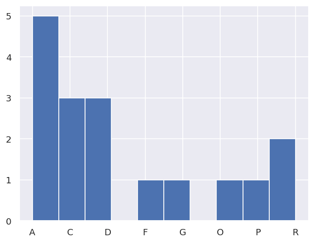
10.5. Classify candidate sets#
To probe the minima found, the classifyFits method can be used. This bins results into “candidate” groups, which can then be examined in detail.
# Run with defaults
# data.classifyFits()
# For more control, pass bins
# Here the minima is set at one end, and a %age range used for bins
minVal = data.fitsSummary['Stats']['redchi']['min']
binRangePC = 1e-5
data.classifyFits(bins = [minVal, minVal + binRangePC*minVal , 20])
| success | chisqr | redchi | ||||||||||
|---|---|---|---|---|---|---|---|---|---|---|---|---|
| count | unique | top | freq | count | unique | top | freq | count | unique | top | freq | |
| redchiGroup | ||||||||||||
| A | 5 | 1 | True | 5 | 5.0 | 5.0 | 0.0 | 1.0 | 5.0 | 5.0 | 0.0 | 1.0 |
| B | 0 | 0 | NaN | NaN | 0 | 0 | NaN | NaN | 0 | 0 | NaN | NaN |
| C | 3 | 1 | True | 3 | 3.0 | 3.0 | 0.0 | 1.0 | 3.0 | 3.0 | 0.0 | 1.0 |
| D | 3 | 1 | True | 3 | 3.0 | 3.0 | 0.0 | 1.0 | 3.0 | 3.0 | 0.0 | 1.0 |
| E | 0 | 0 | NaN | NaN | 0 | 0 | NaN | NaN | 0 | 0 | NaN | NaN |
| F | 1 | 1 | True | 1 | 1.0 | 1.0 | 0.0 | 1.0 | 1.0 | 1.0 | 0.0 | 1.0 |
| G | 1 | 1 | True | 1 | 1.0 | 1.0 | 0.0 | 1.0 | 1.0 | 1.0 | 0.0 | 1.0 |
| H | 0 | 0 | NaN | NaN | 0 | 0 | NaN | NaN | 0 | 0 | NaN | NaN |
| I | 0 | 0 | NaN | NaN | 0 | 0 | NaN | NaN | 0 | 0 | NaN | NaN |
| J | 0 | 0 | NaN | NaN | 0 | 0 | NaN | NaN | 0 | 0 | NaN | NaN |
| K | 0 | 0 | NaN | NaN | 0 | 0 | NaN | NaN | 0 | 0 | NaN | NaN |
| L | 0 | 0 | NaN | NaN | 0 | 0 | NaN | NaN | 0 | 0 | NaN | NaN |
| M | 0 | 0 | NaN | NaN | 0 | 0 | NaN | NaN | 0 | 0 | NaN | NaN |
| N | 0 | 0 | NaN | NaN | 0 | 0 | NaN | NaN | 0 | 0 | NaN | NaN |
| O | 1 | 1 | True | 1 | 1.0 | 1.0 | 0.0 | 1.0 | 1.0 | 1.0 | 0.0 | 1.0 |
| P | 1 | 1 | True | 1 | 1.0 | 1.0 | 0.0 | 1.0 | 1.0 | 1.0 | 0.0 | 1.0 |
| Q | 0 | 0 | NaN | NaN | 0 | 0 | NaN | NaN | 0 | 0 | NaN | NaN |
| R | 2 | 1 | True | 2 | 2.0 | 2.0 | 0.0 | 1.0 | 2.0 | 2.0 | 0.0 | 1.0 |
| S | 0 | 0 | NaN | NaN | 0 | 0 | NaN | NaN | 0 | 0 | NaN | NaN |
*** Warning: found MultiIndex for DataFrame data.index - checkDims may have issues with Pandas MultiIndex, but will try anyway.
*** Warning: found MultiIndex for DataFrame data.index - checkDims may have issues with Pandas MultiIndex, but will try anyway.
10.6. Explore candidate result sets#
Drill-down on a candidate set of results, and examine values and spreads. For more details see PEMtk documentation [20], especially the analysis routines page. (See also Sect. 2.3 for details on the plotting libaries implemented here.)
10.6.1. Raw results#
Plot spreads in magnitude and phase parameters. Statistical plots are available for Seaborn and Holoviews backends, with some slightly different options.
# From the candidates, select a group for analysis
selGroup = 'A'
# paramPlot can be used to check the spread on each parameter.
# Plots use Seaborn or Holoviews/Bokeh
# Colour-mapping is controlled by the 'hue' paramter, additionally pass hRound for sig. fig control.
# The remap setting allows for short-hand labels as set in data.lmmu
paramType = 'm' # Set for (m)agnitude or (p)hase parameters
hRound = 14 # Set for cmapping, default may be too small (leads to all grey cmap on points)
data.paramPlot(selectors={'Type':paramType, 'redchiGroup':selGroup}, hue = 'redchi',
backend=paramPlotBackend, hvType='violin',
returnFlag = True, hRound=hRound, remap = 'lmMap');
*** Warning: found MultiIndex for DataFrame data.index - checkDims may have issues with Pandas MultiIndex, but will try anyway.
paramType = 'p' # Set for (m)agnitude or (p)hase parameters
data.paramPlot(selectors={'Type':paramType, 'redchiGroup':selGroup}, hue = 'redchi', backend=paramPlotBackend, hvType='violin',
returnFlag = True, hRound=hRound, remap = 'lmMap');
*** Warning: found MultiIndex for DataFrame data.index - checkDims may have issues with Pandas MultiIndex, but will try anyway.
10.6.2. Phases, phase shifts & corrections#
Depending on how the fit was configured, phases may be defined in different ways. To set the phases relative to a speific parameter, and wrap to a specified range, use the phaseCorrection() method. This defaults to using the first parameter as a reference phase, and wraps to \(-\pi:\pi\). The phase-corrected values are output to a new Type, ‘pc’, and a set of normalised magnitudes to ‘n’. Additional settings can be passed for more control, as shown below.
# Run phase correction routine
# Set absFlag=True for unsigned phases (mapped to 0:pi)
# Set useRef=False to set ref phase as 0, otherwise the reference value is set.
phaseCorrParams={'absFlag':True, 'useRef':False}
data.phaseCorrection(**phaseCorrParams)
Show code cell output
*** Warning: found MultiIndex for DataFrame data.index - checkDims may have issues with Pandas MultiIndex, but will try anyway.
*** Warning: found MultiIndex for DataFrame data.index - checkDims may have issues with Pandas MultiIndex, but will try anyway.
Set ref param = AG_B3U_B3U_0_0_1_1
| Param | AG_B3U_B3U_0_0_1_1 | AG_B3U_B3U_0_0_n1_1 | AG_B3U_B3U_2_0_1_1 | AG_B3U_B3U_2_0_n1_1 | AG_B3U_B3U_2_2_1_1 | AG_B3U_B3U_2_2_n1_1 | AG_B3U_B3U_2_n2_1_1 | AG_B3U_B3U_2_n2_n1_1 | AG_B3U_B3U_4_0_1_1 | AG_B3U_B3U_4_0_n1_1 | ... | B1G_B3U_B2U_4_n2_1_1 | B1G_B3U_B2U_4_n2_n1_1 | B1G_B3U_B2U_4_n4_1_1 | B1G_B3U_B2U_4_n4_n1_1 | B2G_B3U_B1U_2_1_0_1 | B2G_B3U_B1U_2_n1_0_1 | B2G_B3U_B1U_4_1_0_1 | B2G_B3U_B1U_4_3_0_1 | B2G_B3U_B1U_4_n1_0_1 | B2G_B3U_B1U_4_n3_0_1 | ||
|---|---|---|---|---|---|---|---|---|---|---|---|---|---|---|---|---|---|---|---|---|---|---|---|
| Fit | Type | redchiGroup | |||||||||||||||||||||
| 3 | m | D | 1.414e+00 | 1.414e+00 | 1.961e+00 | 1.961e+00 | 0.811 | 0.811 | 0.811 | 0.811 | 1.005e+00 | 1.005e+00 | ... | 8.665e-01 | 8.665e-01 | 1.571e+00 | 1.571e+00 | 2.000 | 2.000 | 1.850e+00 | 6.151e-01 | 1.850 | 6.151e-01 |
| n | D | 1.789e-01 | 1.789e-01 | 2.481e-01 | 2.481e-01 | 0.103 | 0.103 | 0.103 | 0.103 | 1.272e-01 | 1.272e-01 | ... | 1.096e-01 | 1.096e-01 | 1.988e-01 | 1.988e-01 | 0.253 | 0.253 | 2.340e-01 | 7.781e-02 | 0.234 | 7.781e-02 | |
| p | D | 8.874e-01 | -2.978e+00 | -3.142e+00 | 8.921e-01 | 1.771 | 3.122 | 1.771 | 3.122 | 2.176e+00 | -8.378e-01 | ... | -3.129e+00 | -3.129e+00 | 1.767e+00 | 1.767e+00 | -2.359 | 2.287 | -3.142e+00 | -1.406e+00 | 1.573 | -3.142e+00 | |
| pc | D | 0.000e+00 | 2.417e+00 | 2.254e+00 | 4.709e-03 | 0.884 | 2.234 | 0.884 | 2.234 | 1.288e+00 | 1.725e+00 | ... | 2.267e+00 | 2.267e+00 | 8.797e-01 | 8.797e-01 | 3.037 | 1.399 | 2.254e+00 | 2.293e+00 | 0.686 | 2.254e+00 | |
| 21 | m | R | 2.174e-03 | 2.174e-03 | 1.231e+00 | 1.231e+00 | 1.546 | 1.546 | 1.546 | 1.546 | 6.103e-01 | 6.103e-01 | ... | 4.653e-02 | 4.653e-02 | 2.000e+00 | 2.000e+00 | 1.453 | 1.453 | 3.971e-01 | 1.058e+00 | 0.397 | 1.058e+00 |
| n | R | 3.097e-04 | 3.097e-04 | 1.754e-01 | 1.754e-01 | 0.220 | 0.220 | 0.220 | 0.220 | 8.693e-02 | 8.693e-02 | ... | 6.627e-03 | 6.627e-03 | 2.849e-01 | 2.849e-01 | 0.207 | 0.207 | 5.657e-02 | 1.506e-01 | 0.057 | 1.506e-01 | |
| p | R | 2.748e+00 | -2.978e+00 | -3.141e+00 | -1.419e+00 | -1.034 | 1.706 | -1.034 | 1.706 | 5.541e-03 | 2.703e+00 | ... | -2.539e+00 | -2.539e+00 | -1.571e+00 | -1.571e+00 | -0.101 | 2.024 | -2.944e+00 | -2.127e+00 | 0.778 | -1.525e+00 | |
| pc | R | 0.000e+00 | 5.572e-01 | 3.945e-01 | 2.116e+00 | 2.502 | 1.042 | 2.502 | 1.042 | 2.742e+00 | 4.506e-02 | ... | 9.968e-01 | 9.968e-01 | 1.965e+00 | 1.965e+00 | 2.849 | 0.724 | 5.913e-01 | 1.408e+00 | 1.969 | 2.010e+00 | |
| 29 | m | D | 1.731e+00 | 1.731e+00 | 1.920e+00 | 1.920e+00 | 1.996 | 1.996 | 1.996 | 1.996 | 1.036e+00 | 1.036e+00 | ... | 3.519e-01 | 3.519e-01 | 2.000e+00 | 2.000e+00 | 0.717 | 0.717 | 1.069e-01 | 1.436e+00 | 0.107 | 1.436e+00 |
| n | D | 1.973e-01 | 1.973e-01 | 2.189e-01 | 2.189e-01 | 0.228 | 0.228 | 0.228 | 0.228 | 1.182e-01 | 1.182e-01 | ... | 4.011e-02 | 4.011e-02 | 2.280e-01 | 2.280e-01 | 0.082 | 0.082 | 1.219e-02 | 1.637e-01 | 0.012 | 1.637e-01 | |
| p | D | -2.009e+00 | -2.978e+00 | 9.527e-01 | -1.961e-01 | -2.261 | 0.817 | -2.261 | 0.817 | 2.674e+00 | 2.229e+00 | ... | -2.346e+00 | -2.346e+00 | 3.142e+00 | 3.142e+00 | 3.142 | -0.794 | 3.142e+00 | 2.647e+00 | 0.945 | 1.099e+00 | |
| pc | D | 0.000e+00 | 9.695e-01 | 2.962e+00 | 1.813e+00 | 0.252 | 2.826 | 0.252 | 2.826 | 1.600e+00 | 2.046e+00 | ... | 3.369e-01 | 3.369e-01 | 1.133e+00 | 1.133e+00 | 1.133 | 1.215 | 1.133e+00 | 1.627e+00 | 2.954 | 3.108e+00 | |
| 62 | m | O | 1.993e+00 | 1.993e+00 | 1.510e+00 | 1.510e+00 | 0.202 | 0.202 | 0.202 | 0.202 | 2.868e-01 | 2.868e-01 | ... | 1.959e+00 | 1.959e+00 | 2.402e-01 | 2.402e-01 | 0.616 | 0.616 | 1.920e-01 | 5.124e-01 | 0.192 | 5.124e-01 |
| n | O | 2.679e-01 | 2.679e-01 | 2.030e-01 | 2.030e-01 | 0.027 | 0.027 | 0.027 | 0.027 | 3.856e-02 | 3.856e-02 | ... | 2.633e-01 | 2.633e-01 | 3.230e-02 | 3.230e-02 | 0.083 | 0.083 | 2.581e-02 | 6.888e-02 | 0.026 | 6.888e-02 | |
| p | O | -7.141e-01 | -2.978e+00 | -3.041e+00 | -7.395e-01 | -2.727 | 2.764 | -2.727 | 2.764 | 3.088e-01 | -3.142e+00 | ... | 1.963e+00 | 1.963e+00 | -3.132e+00 | -3.132e+00 | 0.486 | 3.141 | 1.462e+00 | 2.004e+00 | -3.142 | 5.058e-01 | |
| pc | O | 0.000e+00 | 2.264e+00 | 2.327e+00 | 2.535e-02 | 2.013 | 2.805 | 2.013 | 2.805 | 1.023e+00 | 2.427e+00 | ... | 2.677e+00 | 2.677e+00 | 2.418e+00 | 2.418e+00 | 1.201 | 2.428 | 2.176e+00 | 2.718e+00 | 2.427 | 1.220e+00 | |
| 98 | m | D | 1.954e+00 | 1.954e+00 | 1.795e+00 | 1.795e+00 | 1.542 | 1.542 | 1.542 | 1.542 | 9.707e-01 | 9.707e-01 | ... | 1.349e-01 | 1.349e-01 | 2.914e-03 | 2.914e-03 | 0.749 | 0.749 | 1.244e+00 | 1.351e-03 | 1.244 | 1.351e-03 |
| n | D | 2.484e-01 | 2.484e-01 | 2.282e-01 | 2.282e-01 | 0.196 | 0.196 | 0.196 | 0.196 | 1.234e-01 | 1.234e-01 | ... | 1.715e-02 | 1.715e-02 | 3.704e-04 | 3.704e-04 | 0.095 | 0.095 | 1.581e-01 | 1.717e-04 | 0.158 | 1.717e-04 | |
| p | D | -1.712e+00 | -2.978e+00 | -2.940e+00 | -1.101e+00 | 0.272 | 3.135 | 0.272 | 3.135 | 2.087e+00 | -2.322e+00 | ... | 4.808e-01 | 4.808e-01 | -2.534e+00 | -2.534e+00 | 2.111 | -0.066 | -3.142e+00 | -2.832e+00 | 1.570 | -2.458e+00 | |
| pc | D | 0.000e+00 | 1.266e+00 | 1.228e+00 | 6.112e-01 | 1.984 | 1.437 | 1.984 | 1.437 | 2.485e+00 | 6.099e-01 | ... | 2.193e+00 | 2.193e+00 | 8.215e-01 | 8.215e-01 | 2.461 | 1.646 | 1.430e+00 | 1.120e+00 | 3.001 | 7.463e-01 | |
| 169 | m | A | 1.306e-01 | 1.306e-01 | 1.007e-04 | 1.007e-04 | 1.360 | 1.360 | 1.360 | 1.360 | 5.800e-01 | 5.800e-01 | ... | 2.044e-02 | 2.044e-02 | 3.776e-01 | 3.776e-01 | 1.603 | 1.603 | 2.628e-01 | 9.623e-01 | 0.263 | 9.623e-01 |
| n | A | 2.260e-02 | 2.260e-02 | 1.742e-05 | 1.742e-05 | 0.235 | 0.235 | 0.235 | 0.235 | 1.004e-01 | 1.004e-01 | ... | 3.537e-03 | 3.537e-03 | 6.534e-02 | 6.534e-02 | 0.277 | 0.277 | 4.547e-02 | 1.665e-01 | 0.045 | 1.665e-01 | |
| p | A | 3.137e+00 | -2.978e+00 | 1.134e+00 | -2.687e+00 | -2.239 | 1.256 | -2.239 | 1.256 | -1.147e+00 | 1.149e+00 | ... | -2.510e+00 | -2.510e+00 | -1.455e+00 | -1.455e+00 | 2.395 | 0.845 | -8.323e-01 | 2.437e+00 | -0.371 | 3.750e-01 | |
| pc | A | 0.000e+00 | 1.676e-01 | 2.003e+00 | 4.587e-01 | 0.907 | 1.881 | 0.907 | 1.881 | 1.999e+00 | 1.988e+00 | ... | 6.359e-01 | 6.359e-01 | 1.691e+00 | 1.691e+00 | 0.742 | 2.292 | 2.314e+00 | 6.998e-01 | 2.775 | 2.762e+00 | |
| 171 | m | A | 1.944e-02 | 1.944e-02 | 1.773e+00 | 1.773e+00 | 1.650 | 1.650 | 1.650 | 1.650 | 5.698e-01 | 5.698e-01 | ... | 9.824e-03 | 9.824e-03 | 9.877e-01 | 9.877e-01 | 0.308 | 0.308 | 9.073e-01 | 1.897e+00 | 0.907 | 1.897e+00 |
| n | A | 2.573e-03 | 2.573e-03 | 2.347e-01 | 2.347e-01 | 0.218 | 0.218 | 0.218 | 0.218 | 7.544e-02 | 7.544e-02 | ... | 1.301e-03 | 1.301e-03 | 1.308e-01 | 1.308e-01 | 0.041 | 0.041 | 1.201e-01 | 2.511e-01 | 0.120 | 2.511e-01 | |
| p | A | -5.230e-01 | -2.978e+00 | 1.188e+00 | -1.968e+00 | 3.082 | -0.859 | 3.082 | -0.859 | -4.008e-01 | 1.051e+00 | ... | 1.722e+00 | 1.722e+00 | -2.675e+00 | -2.675e+00 | -0.465 | 2.862 | -1.611e+00 | -2.838e+00 | -3.136 | 1.800e+00 | |
| pc | A | 0.000e+00 | 2.455e+00 | 1.711e+00 | 1.445e+00 | 2.678 | 0.336 | 2.678 | 0.336 | 1.222e-01 | 1.574e+00 | ... | 2.245e+00 | 2.245e+00 | 2.152e+00 | 2.152e+00 | 0.058 | 2.899 | 1.088e+00 | 2.315e+00 | 2.613 | 2.323e+00 | |
| 177 | m | F | 1.956e+00 | 1.956e+00 | 1.104e+00 | 1.104e+00 | 1.925 | 1.925 | 1.925 | 1.925 | 8.990e-01 | 8.990e-01 | ... | 7.198e-01 | 7.198e-01 | 5.837e-01 | 5.837e-01 | 0.296 | 0.296 | 9.463e-01 | 6.881e-01 | 0.946 | 6.881e-01 |
| n | F | 2.672e-01 | 2.672e-01 | 1.508e-01 | 1.508e-01 | 0.263 | 0.263 | 0.263 | 0.263 | 1.228e-01 | 1.228e-01 | ... | 9.831e-02 | 9.831e-02 | 7.973e-02 | 7.973e-02 | 0.040 | 0.040 | 1.293e-01 | 9.400e-02 | 0.129 | 9.400e-02 | |
| p | F | -9.895e-01 | -2.978e+00 | -3.097e+00 | 1.328e-01 | -0.311 | -2.019 | -0.311 | -2.019 | 3.140e+00 | 1.401e+00 | ... | -1.949e+00 | -1.949e+00 | -2.237e+00 | -2.237e+00 | 0.856 | -1.003 | 3.142e+00 | 2.715e+00 | -1.625 | -1.183e+00 | |
| pc | F | 0.000e+00 | 1.989e+00 | 2.108e+00 | 1.122e+00 | 0.679 | 1.029 | 0.679 | 1.029 | 2.153e+00 | 2.391e+00 | ... | 9.599e-01 | 9.599e-01 | 1.248e+00 | 1.248e+00 | 1.846 | 0.013 | 2.152e+00 | 2.579e+00 | 0.636 | 1.933e-01 | |
| 182 | m | G | 1.999e+00 | 1.999e+00 | 1.670e+00 | 1.670e+00 | 0.844 | 0.844 | 0.844 | 0.844 | 1.280e+00 | 1.280e+00 | ... | 7.613e-02 | 7.613e-02 | 3.333e-04 | 3.333e-04 | 0.694 | 0.694 | 4.347e-01 | 2.664e-01 | 0.435 | 2.664e-01 |
| n | G | 3.703e-01 | 3.703e-01 | 3.094e-01 | 3.094e-01 | 0.156 | 0.156 | 0.156 | 0.156 | 2.372e-01 | 2.372e-01 | ... | 1.410e-02 | 1.410e-02 | 6.173e-05 | 6.173e-05 | 0.128 | 0.128 | 8.052e-02 | 4.934e-02 | 0.081 | 4.934e-02 | |
| p | G | -9.043e-02 | -2.978e+00 | 3.138e+00 | 3.805e-01 | -0.317 | 3.142 | -0.317 | 3.142 | 1.157e+00 | -2.562e+00 | ... | 3.142e+00 | 3.142e+00 | -2.679e+00 | -2.679e+00 | 0.935 | 3.136 | 1.710e+00 | -1.893e+00 | -3.032 | 2.169e+00 | |
| pc | G | 0.000e+00 | 2.888e+00 | 3.055e+00 | 4.710e-01 | 0.226 | 3.051 | 0.226 | 3.051 | 1.248e+00 | 2.471e+00 | ... | 3.051e+00 | 3.051e+00 | 2.588e+00 | 2.588e+00 | 1.026 | 3.057 | 1.800e+00 | 1.802e+00 | 2.942 | 2.260e+00 | |
| 187 | m | C | 3.609e-01 | 3.609e-01 | 5.147e-01 | 5.147e-01 | 1.607 | 1.607 | 1.607 | 1.607 | 1.388e+00 | 1.388e+00 | ... | 1.271e-01 | 1.271e-01 | 2.000e+00 | 2.000e+00 | 0.611 | 0.611 | 1.529e+00 | 5.298e-02 | 1.529 | 5.298e-02 |
| n | C | 5.289e-02 | 5.289e-02 | 7.542e-02 | 7.542e-02 | 0.235 | 0.235 | 0.235 | 0.235 | 2.034e-01 | 2.034e-01 | ... | 1.862e-02 | 1.862e-02 | 2.931e-01 | 2.931e-01 | 0.090 | 0.090 | 2.241e-01 | 7.764e-03 | 0.224 | 7.764e-03 | |
| p | C | 2.916e+00 | -2.978e+00 | -1.156e-01 | 2.260e+00 | 2.486 | -1.401 | 2.486 | -1.401 | -2.086e+00 | 6.817e-02 | ... | -2.532e+00 | -2.532e+00 | 1.795e+00 | 1.795e+00 | -0.749 | 2.936 | -1.182e+00 | -2.700e-01 | 0.389 | 1.438e+00 | |
| pc | C | 0.000e+00 | 3.890e-01 | 3.031e+00 | 6.554e-01 | 0.430 | 1.966 | 0.430 | 1.966 | 1.281e+00 | 2.848e+00 | ... | 8.357e-01 | 8.357e-01 | 1.120e+00 | 1.120e+00 | 2.619 | 0.021 | 2.185e+00 | 3.097e+00 | 2.527 | 1.478e+00 | |
| 205 | m | P | 5.801e-02 | 5.801e-02 | 2.000e+00 | 2.000e+00 | 1.731 | 1.731 | 1.731 | 1.731 | 7.411e-02 | 7.411e-02 | ... | 1.202e+00 | 1.202e+00 | 1.491e+00 | 1.491e+00 | 1.273 | 1.273 | 4.799e-01 | 4.870e-01 | 0.480 | 4.870e-01 |
| n | P | 6.268e-03 | 6.268e-03 | 2.161e-01 | 2.161e-01 | 0.187 | 0.187 | 0.187 | 0.187 | 8.008e-03 | 8.008e-03 | ... | 1.299e-01 | 1.299e-01 | 1.611e-01 | 1.611e-01 | 0.138 | 0.138 | 5.185e-02 | 5.262e-02 | 0.052 | 5.262e-02 | |
| p | P | -3.142e+00 | -2.978e+00 | 2.173e-01 | 9.302e-01 | 2.841 | 1.367 | 2.841 | 1.367 | 1.774e+00 | -1.966e+00 | ... | -2.284e+00 | -2.284e+00 | 1.033e-02 | 1.033e-02 | -2.920 | -1.247 | -3.142e+00 | -1.252e+00 | 1.687 | 1.196e+00 | |
| pc | P | 0.000e+00 | 1.632e-01 | 2.924e+00 | 2.212e+00 | 0.300 | 1.775 | 0.300 | 1.775 | 1.368e+00 | 1.175e+00 | ... | 8.575e-01 | 8.575e-01 | 3.131e+00 | 3.131e+00 | 0.222 | 1.895 | 7.498e-05 | 1.889e+00 | 1.455 | 1.946e+00 | |
| 240 | m | A | 2.000e+00 | 2.000e+00 | 1.110e+00 | 1.110e+00 | 1.842 | 1.842 | 1.842 | 1.842 | 1.135e+00 | 1.135e+00 | ... | 5.217e-01 | 5.217e-01 | 2.505e-03 | 2.505e-03 | 0.566 | 0.566 | 2.973e-01 | 4.915e-02 | 0.297 | 4.915e-02 |
| n | A | 3.596e-01 | 3.596e-01 | 1.996e-01 | 1.996e-01 | 0.331 | 0.331 | 0.331 | 0.331 | 2.041e-01 | 2.041e-01 | ... | 9.379e-02 | 9.379e-02 | 4.503e-04 | 4.503e-04 | 0.102 | 0.102 | 5.344e-02 | 8.836e-03 | 0.053 | 8.836e-03 | |
| p | A | -3.132e-01 | -2.978e+00 | 3.141e+00 | 2.409e-01 | -0.577 | 2.763 | -0.577 | 2.763 | 3.870e-01 | 3.051e+00 | ... | -1.371e+00 | -1.371e+00 | -6.182e-02 | -6.182e-02 | -1.628 | 1.400 | -1.842e+00 | 3.103e+00 | -0.267 | -5.159e-01 | |
| pc | A | 0.000e+00 | 2.665e+00 | 2.829e+00 | 5.541e-01 | 0.264 | 3.076 | 0.264 | 3.076 | 7.002e-01 | 2.919e+00 | ... | 1.058e+00 | 1.058e+00 | 2.513e-01 | 2.513e-01 | 1.315 | 1.713 | 1.528e+00 | 2.867e+00 | 0.046 | 2.028e-01 | |
| 257 | m | C | 1.963e+00 | 1.963e+00 | 2.000e+00 | 2.000e+00 | 1.242 | 1.242 | 1.242 | 1.242 | 8.810e-01 | 8.810e-01 | ... | 6.081e-01 | 6.081e-01 | 2.152e-01 | 2.152e-01 | 1.556 | 1.556 | 1.408e-01 | 6.595e-01 | 0.141 | 6.595e-01 |
| n | C | 2.527e-01 | 2.527e-01 | 2.574e-01 | 2.574e-01 | 0.160 | 0.160 | 0.160 | 0.160 | 1.134e-01 | 1.134e-01 | ... | 7.826e-02 | 7.826e-02 | 2.770e-02 | 2.770e-02 | 0.200 | 0.200 | 1.812e-02 | 8.488e-02 | 0.018 | 8.488e-02 | |
| p | C | -1.014e+00 | -2.978e+00 | 4.223e-01 | -2.235e+00 | -0.006 | 2.666 | -0.006 | 2.666 | -2.013e+00 | 6.392e-01 | ... | 2.108e+00 | 2.108e+00 | -1.123e+00 | -1.123e+00 | 1.151 | -0.504 | -2.900e+00 | -6.288e-01 | 3.018 | 1.256e+00 | |
| pc | C | 0.000e+00 | 1.965e+00 | 1.436e+00 | 1.221e+00 | 1.008 | 2.604 | 1.008 | 2.604 | 9.994e-01 | 1.653e+00 | ... | 3.122e+00 | 3.122e+00 | 1.092e-01 | 1.092e-01 | 2.165 | 0.509 | 1.886e+00 | 3.847e-01 | 2.252 | 2.269e+00 | |
| 313 | m | A | 1.810e+00 | 1.810e+00 | 3.956e-01 | 3.956e-01 | 1.694 | 1.694 | 1.694 | 1.694 | 1.000e-04 | 1.000e-04 | ... | 1.000e-04 | 1.000e-04 | 1.164e-04 | 1.164e-04 | 0.612 | 0.612 | 6.460e-01 | 9.270e-01 | 0.646 | 9.270e-01 |
| n | A | 2.408e-01 | 2.408e-01 | 5.262e-02 | 5.262e-02 | 0.225 | 0.225 | 0.225 | 0.225 | 1.330e-05 | 1.330e-05 | ... | 1.330e-05 | 1.330e-05 | 1.547e-05 | 1.547e-05 | 0.081 | 0.081 | 8.592e-02 | 1.233e-01 | 0.086 | 1.233e-01 | |
| p | A | 3.139e+00 | -2.978e+00 | 2.264e-01 | -3.142e+00 | -2.028 | 1.934 | -2.028 | 1.934 | 3.051e+00 | 3.140e+00 | ... | 2.106e+00 | 2.106e+00 | 2.846e+00 | 2.846e+00 | 1.381 | 1.651 | -9.065e-01 | 3.901e-01 | -2.203 | -3.142e+00 | |
| pc | A | 0.000e+00 | 1.663e-01 | 2.912e+00 | 3.032e-03 | 1.117 | 1.205 | 1.117 | 1.205 | 8.750e-02 | 1.011e-03 | ... | 1.033e+00 | 1.033e+00 | 2.923e-01 | 2.923e-01 | 1.757 | 1.488 | 2.238e+00 | 2.748e+00 | 0.942 | 3.117e-03 | |
| 327 | m | R | 8.312e-01 | 8.312e-01 | 7.110e-01 | 7.110e-01 | 1.988 | 1.988 | 1.988 | 1.988 | 8.993e-01 | 8.993e-01 | ... | 5.906e-01 | 5.906e-01 | 1.999e+00 | 1.999e+00 | 0.947 | 0.947 | 7.137e-02 | 1.068e+00 | 0.071 | 1.068e+00 |
| n | R | 1.282e-01 | 1.282e-01 | 1.097e-01 | 1.097e-01 | 0.307 | 0.307 | 0.307 | 0.307 | 1.388e-01 | 1.388e-01 | ... | 9.112e-02 | 9.112e-02 | 3.084e-01 | 3.084e-01 | 0.146 | 0.146 | 1.101e-02 | 1.648e-01 | 0.011 | 1.648e-01 | |
| p | R | 2.742e+00 | -2.978e+00 | -3.142e+00 | 3.142e+00 | 0.165 | -2.312 | 0.165 | -2.312 | -2.597e-01 | 1.650e-01 | ... | 2.328e+00 | 2.328e+00 | 2.442e-02 | 2.442e-02 | -1.057 | 0.901 | -1.695e+00 | 2.358e-01 | 1.499 | -1.315e+00 | |
| pc | R | 0.000e+00 | 5.631e-01 | 3.998e-01 | 3.998e-01 | 2.577 | 1.230 | 2.577 | 1.230 | 3.001e+00 | 2.577e+00 | ... | 4.134e-01 | 4.134e-01 | 2.717e+00 | 2.717e+00 | 2.485 | 1.840 | 1.846e+00 | 2.506e+00 | 1.243 | 2.227e+00 | |
| 362 | m | C | 9.163e-01 | 9.163e-01 | 5.789e-04 | 5.789e-04 | 1.365 | 1.365 | 1.365 | 1.365 | 1.490e+00 | 1.490e+00 | ... | 9.014e-02 | 9.014e-02 | 1.064e+00 | 1.064e+00 | 0.561 | 0.561 | 3.857e-01 | 1.419e-01 | 0.386 | 1.419e-01 |
| n | C | 1.395e-01 | 1.395e-01 | 8.815e-05 | 8.815e-05 | 0.208 | 0.208 | 0.208 | 0.208 | 2.268e-01 | 2.268e-01 | ... | 1.373e-02 | 1.373e-02 | 1.621e-01 | 1.621e-01 | 0.085 | 0.085 | 5.873e-02 | 2.160e-02 | 0.059 | 2.160e-02 | |
| p | C | 2.457e+00 | -2.978e+00 | -2.317e-01 | 9.804e-01 | -0.525 | -3.141 | -0.525 | -3.141 | -1.293e+00 | 3.378e-01 | ... | -6.110e-01 | -6.110e-01 | -2.248e-01 | -2.248e-01 | 0.153 | -3.115 | -1.832e+00 | 1.096e+00 | 2.886 | -3.141e+00 | |
| pc | C | 0.000e+00 | 8.483e-01 | 2.688e+00 | 1.476e+00 | 2.982 | 0.685 | 2.982 | 0.685 | 2.534e+00 | 2.119e+00 | ... | 3.068e+00 | 3.068e+00 | 2.681e+00 | 2.681e+00 | 2.304 | 0.712 | 1.995e+00 | 1.361e+00 | 0.429 | 6.855e-01 | |
| 370 | m | A | 1.935e+00 | 1.935e+00 | 1.017e+00 | 1.017e+00 | 1.628 | 1.628 | 1.628 | 1.628 | 1.496e+00 | 1.496e+00 | ... | 8.391e-02 | 8.391e-02 | 2.607e-01 | 2.607e-01 | 0.851 | 0.851 | 1.736e-01 | 3.487e-01 | 0.174 | 3.487e-01 |
| n | A | 3.106e-01 | 3.106e-01 | 1.633e-01 | 1.633e-01 | 0.261 | 0.261 | 0.261 | 0.261 | 2.402e-01 | 2.402e-01 | ... | 1.347e-02 | 1.347e-02 | 4.186e-02 | 4.186e-02 | 0.137 | 0.137 | 2.788e-02 | 5.598e-02 | 0.028 | 5.598e-02 | |
| p | A | 1.345e+00 | -2.978e+00 | 2.551e+00 | 7.043e-02 | -0.022 | -3.028 | -0.022 | -3.028 | 2.070e+00 | -2.611e+00 | ... | 3.142e+00 | 3.142e+00 | 1.757e+00 | 1.757e+00 | -0.748 | -2.865 | 1.658e+00 | -1.728e+00 | -2.716 | -7.260e-01 | |
| pc | A | 0.000e+00 | 1.960e+00 | 1.206e+00 | 1.275e+00 | 1.368 | 1.910 | 1.368 | 1.910 | 7.248e-01 | 2.327e+00 | ... | 1.796e+00 | 1.796e+00 | 4.120e-01 | 4.120e-01 | 2.093 | 2.073 | 3.133e-01 | 3.073e+00 | 2.222 | 2.071e+00 |
68 rows × 38 columns
Examine new data types…
paramType = 'n'
data.paramPlot(selectors={'Type':paramType, 'redchiGroup':selGroup}, hue = 'redchi',
backend=paramPlotBackend, hvType='violin', kind='box',
returnFlag = True, hRound=hRound, remap = 'lmMap');
*** Warning: found MultiIndex for DataFrame data.index - checkDims may have issues with Pandas MultiIndex, but will try anyway.
WARNING:param.Scatter10529: Setting non-parameter attribute kind=box using a mechanism intended only for parameters
paramType = 'pc'
data.paramPlot(selectors={'Type':paramType, 'redchiGroup':selGroup}, hue = 'redchi',
backend=paramPlotBackend, hvType='violin', kind='box',
returnFlag = True, hRound=hRound, remap = 'lmMap');
*** Warning: found MultiIndex for DataFrame data.index - checkDims may have issues with Pandas MultiIndex, but will try anyway.
WARNING:param.Scatter11149: Setting non-parameter attribute kind=box using a mechanism intended only for parameters
10.7. Parameter estimation & fidelity#
For case studies, the fit results can be directly compared to the known input parameters. This should give a feel for how well the data defines the matrix elements (parameters) in this case. In general, probing the correlations and spread of results, and comparing to other (unfitted) results is required to estimate fidelity, see Quantum Metrology Vols. 1 & 2 [4, 9] for further discussion.
10.7.1. Best values and statistics#
To get a final parameter set and associated statistics, based on a subset of the fit results, the paramsReport() method is available. If reference data is available, as for the case studies herein, the paramsCompare() method can also be used to compare with the reference case.
# Parameter summary
data.paramsReport(inds = {'redchiGroup':selGroup})
Show code cell output
*** Warning: found MultiIndex for DataFrame data.index - checkDims may have issues with Pandas MultiIndex, but will try anyway.
Set parameter stats to self.paramsSummary.
| Type | m | n | p | pc | |
|---|---|---|---|---|---|
| Param | Agg | ||||
| AG_B3U_B3U_0_0_1_1 | min | 0.019 | 0.003 | -0.523 | 0.000 |
| mean | 1.179 | 0.187 | 1.357 | 0.000 | |
| median | 1.810 | 0.241 | 1.345 | 0.000 | |
| max | 2.000 | 0.360 | 3.139 | 0.000 | |
| std | 1.011 | 0.165 | 1.780 | 0.000 | |
| ... | ... | ... | ... | ... | ... |
| B2G_B3U_B1U_4_n3_0_1 | mean | 0.837 | 0.121 | -0.442 | 1.473 |
| median | 0.927 | 0.123 | -0.516 | 2.071 | |
| max | 1.897 | 0.251 | 1.800 | 2.762 | |
| std | 0.708 | 0.095 | 1.808 | 1.276 | |
| var | 0.502 | 0.009 | 3.267 | 1.629 |
228 rows × 4 columns
# Parameter comparison
# Note this uses phaseCorrParams as set previously for consistency
data.paramsCompare(phaseCorrParams=phaseCorrParams)
Show code cell output
*** Warning: found MultiIndex for DataFrame data.index - checkDims may have issues with Pandas MultiIndex, but will try anyway.
*** Warning: found MultiIndex for DataFrame data.index - checkDims may have issues with Pandas MultiIndex, but will try anyway.
Set ref param = AG_B3U_B3U_0_0_1_1
Set parameter comparison to self.paramsSummaryComp.
| Param | AG_B3U_B3U_0_0_1_1 | AG_B3U_B3U_0_0_n1_1 | AG_B3U_B3U_2_0_1_1 | AG_B3U_B3U_2_0_n1_1 | AG_B3U_B3U_2_2_1_1 | AG_B3U_B3U_2_2_n1_1 | AG_B3U_B3U_2_n2_1_1 | AG_B3U_B3U_2_n2_n1_1 | AG_B3U_B3U_4_0_1_1 | AG_B3U_B3U_4_0_n1_1 | ... | B1G_B3U_B2U_4_n2_1_1 | B1G_B3U_B2U_4_n2_n1_1 | B1G_B3U_B2U_4_n4_1_1 | B1G_B3U_B2U_4_n4_n1_1 | B2G_B3U_B1U_2_1_0_1 | B2G_B3U_B1U_2_n1_0_1 | B2G_B3U_B1U_4_1_0_1 | B2G_B3U_B1U_4_3_0_1 | B2G_B3U_B1U_4_n1_0_1 | B2G_B3U_B1U_4_n3_0_1 | |
|---|---|---|---|---|---|---|---|---|---|---|---|---|---|---|---|---|---|---|---|---|---|---|
| Fit | Type | |||||||||||||||||||||
| ref | m | 1.366 | 1.366 | 1.299 | 1.299 | 1.386 | 1.386 | 1.386 | 1.386 | 0.400 | 0.400 | ... | 0.154 | 0.154 | 0.035 | 0.035 | 0.521 | 0.521 | 0.162 | 0.074 | 0.162 | 0.074 |
| n | 0.268 | 0.268 | 0.255 | 0.255 | 0.272 | 0.272 | 0.272 | 0.272 | 0.079 | 0.079 | ... | 0.030 | 0.030 | 0.007 | 0.007 | 0.102 | 0.102 | 0.032 | 0.015 | 0.032 | 0.015 | |
| p | 0.163 | -2.978 | -2.385 | 0.756 | 0.802 | -2.340 | 0.802 | -2.340 | 2.494 | -0.647 | ... | -2.025 | -2.025 | 0.037 | 0.037 | -0.646 | 2.495 | -1.079 | -1.168 | 2.063 | 1.974 | |
| pc | 0.000 | 3.142 | 2.548 | 0.593 | 0.639 | 2.503 | 0.639 | 2.503 | 2.331 | 0.811 | ... | 2.188 | 2.188 | 0.126 | 0.126 | 0.810 | 2.332 | 1.242 | 1.331 | 1.900 | 1.810 |
4 rows × 38 columns
| Param | AG_B3U_B3U_0_0_1_1 | AG_B3U_B3U_0_0_n1_1 | AG_B3U_B3U_2_0_1_1 | AG_B3U_B3U_2_0_n1_1 | AG_B3U_B3U_2_2_1_1 | AG_B3U_B3U_2_2_n1_1 | AG_B3U_B3U_2_n2_1_1 | AG_B3U_B3U_2_n2_n1_1 | AG_B3U_B3U_4_0_1_1 | AG_B3U_B3U_4_0_n1_1 | ... | B1G_B3U_B2U_4_n2_1_1 | B1G_B3U_B2U_4_n2_n1_1 | B1G_B3U_B2U_4_n4_1_1 | B1G_B3U_B2U_4_n4_n1_1 | B2G_B3U_B1U_2_1_0_1 | B2G_B3U_B1U_2_n1_0_1 | B2G_B3U_B1U_4_1_0_1 | B2G_B3U_B1U_4_3_0_1 | B2G_B3U_B1U_4_n1_0_1 | B2G_B3U_B1U_4_n3_0_1 | ||
|---|---|---|---|---|---|---|---|---|---|---|---|---|---|---|---|---|---|---|---|---|---|---|---|
| Type | Source | dType | |||||||||||||||||||||
| m | mean | num | 1.179 | 1.179 | 0.859 | 0.859 | 1.635 | 1.635 | 1.635 | 1.635 | 0.756 | 0.756 | ... | 0.127 | 0.127 | 0.326 | 0.326 | 0.788 | 0.788 | 0.457 | 0.837 | 0.457 | 0.837 |
| ref | num | 1.366 | 1.366 | 1.299 | 1.299 | 1.386 | 1.386 | 1.386 | 1.386 | 0.400 | 0.400 | ... | 0.154 | 0.154 | 0.035 | 0.035 | 0.521 | 0.521 | 0.162 | 0.074 | 0.162 | 0.074 | |
| diff | % | 15.900 | 15.900 | 51.143 | 51.143 | 15.198 | 15.198 | 15.198 | 15.198 | 47.063 | 47.063 | ... | 20.847 | 20.847 | 89.145 | 89.145 | 33.939 | 33.939 | 64.476 | 91.112 | 64.476 | 91.112 | |
| num | -0.187 | -0.187 | -0.439 | -0.439 | 0.248 | 0.248 | 0.248 | 0.248 | 0.356 | 0.356 | ... | -0.027 | -0.027 | 0.290 | 0.290 | 0.267 | 0.267 | 0.295 | 0.762 | 0.295 | 0.762 | ||
| std | % | 85.738 | 85.738 | 79.694 | 79.694 | 10.684 | 10.684 | 10.684 | 10.684 | 76.209 | 76.209 | ... | 175.285 | 175.285 | 124.290 | 124.290 | 62.750 | 62.750 | 67.565 | 84.633 | 67.565 | 84.633 | |
| num | 1.011 | 1.011 | 0.685 | 0.685 | 0.175 | 0.175 | 0.175 | 0.175 | 0.576 | 0.576 | ... | 0.223 | 0.223 | 0.405 | 0.405 | 0.494 | 0.494 | 0.309 | 0.708 | 0.309 | 0.708 | ||
| diff/std | % | 18.545 | 18.545 | 64.173 | 64.173 | 142.256 | 142.256 | 142.256 | 142.256 | 61.755 | 61.755 | ... | 11.893 | 11.893 | 71.723 | 71.723 | 54.086 | 54.086 | 95.429 | 107.655 | 95.429 | 107.655 | |
| n | mean | num | 0.187 | 0.187 | 0.130 | 0.130 | 0.254 | 0.254 | 0.254 | 0.254 | 0.124 | 0.124 | ... | 0.022 | 0.022 | 0.048 | 0.048 | 0.128 | 0.128 | 0.067 | 0.121 | 0.067 | 0.121 |
| ref | num | 0.268 | 0.268 | 0.255 | 0.255 | 0.272 | 0.272 | 0.272 | 0.272 | 0.079 | 0.079 | ... | 0.030 | 0.030 | 0.007 | 0.007 | 0.102 | 0.102 | 0.032 | 0.015 | 0.032 | 0.015 | |
| diff | % | 43.240 | 43.240 | 95.963 | 95.963 | 6.979 | 6.979 | 6.979 | 6.979 | 36.651 | 36.651 | ... | 34.531 | 34.531 | 85.449 | 85.449 | 19.929 | 19.929 | 52.096 | 87.952 | 52.096 | 87.952 | |
| num | -0.081 | -0.081 | -0.125 | -0.125 | -0.018 | -0.018 | -0.018 | -0.018 | 0.045 | 0.045 | ... | -0.008 | -0.008 | 0.041 | 0.041 | 0.025 | 0.025 | 0.035 | 0.107 | 0.035 | 0.107 | ||
| std | % | 88.166 | 88.166 | 76.703 | 76.703 | 18.057 | 18.057 | 18.057 | 18.057 | 78.802 | 78.802 | ... | 179.484 | 179.484 | 113.665 | 113.665 | 71.017 | 71.017 | 54.975 | 78.110 | 54.975 | 78.110 | |
| num | 0.165 | 0.165 | 0.100 | 0.100 | 0.046 | 0.046 | 0.046 | 0.046 | 0.098 | 0.098 | ... | 0.040 | 0.040 | 0.054 | 0.054 | 0.091 | 0.091 | 0.037 | 0.095 | 0.037 | 0.095 | ||
| diff/std | % | 49.044 | 49.044 | 125.111 | 125.111 | 38.647 | 38.647 | 38.647 | 38.647 | 46.511 | 46.511 | ... | 19.239 | 19.239 | 75.176 | 75.176 | 28.062 | 28.062 | 94.763 | 112.600 | 94.763 | 112.600 | |
| p | mean | num | 1.357 | -2.978 | 1.648 | -1.497 | -0.357 | 0.413 | -0.357 | 0.413 | 0.792 | 1.156 | ... | 0.618 | 0.618 | 0.082 | 0.082 | 0.187 | 0.778 | -0.706 | 0.273 | -1.739 | -0.442 |
| ref | num | 0.163 | -2.978 | -2.385 | 0.756 | 0.802 | -2.340 | 0.802 | -2.340 | 2.494 | -0.647 | ... | -2.025 | -2.025 | 0.037 | 0.037 | -0.646 | 2.495 | -1.079 | -1.168 | 2.063 | 1.974 | |
| diff | % | 87.971 | 0.000 | 244.712 | 150.525 | 324.612 | 666.272 | 324.612 | 666.272 | 214.888 | 156.011 | ... | 427.780 | 427.780 | 54.802 | 54.802 | 445.431 | 220.565 | 52.709 | 528.291 | 218.631 | 546.921 | |
| num | 1.194 | 0.000 | 4.033 | -2.253 | -1.159 | 2.753 | -1.159 | 2.753 | -1.702 | 1.803 | ... | 2.643 | 2.643 | 0.045 | 0.045 | 0.833 | -1.717 | 0.372 | 1.441 | -3.802 | -2.415 | ||
| std | % | 131.140 | 0.000 | 71.415 | 104.662 | 599.642 | 567.657 | 599.642 | 567.657 | 219.427 | 201.629 | ... | 392.707 | 392.707 | 2745.660 | 2745.660 | 882.005 | 278.258 | 197.085 | 941.927 | 76.940 | 409.308 | |
| num | 1.780 | 0.000 | 1.177 | 1.567 | 2.140 | 2.346 | 2.140 | 2.346 | 1.738 | 2.331 | ... | 2.426 | 2.426 | 2.260 | 2.260 | 1.650 | 2.166 | 1.392 | 2.569 | 1.338 | 1.808 | ||
| diff/std | % | 67.082 | NaN | 342.663 | 143.820 | 54.134 | 117.372 | 54.134 | 117.372 | 97.931 | 77.375 | ... | 108.931 | 108.931 | 1.996 | 1.996 | 50.502 | 79.266 | 26.744 | 56.086 | 284.156 | 133.621 | |
| pc | mean | num | 0.000 | 1.483 | 2.132 | 0.747 | 1.267 | 1.682 | 1.267 | 1.682 | 0.727 | 1.762 | ... | 1.354 | 1.354 | 0.960 | 0.960 | 1.193 | 2.093 | 1.496 | 2.341 | 1.719 | 1.473 |
| ref | num | 0.000 | 3.142 | 2.548 | 0.593 | 0.639 | 2.503 | 0.639 | 2.503 | 2.331 | 0.811 | ... | 2.188 | 2.188 | 0.126 | 0.126 | 0.810 | 2.332 | 1.242 | 1.331 | 1.900 | 1.810 | |
| diff | % | NaN | 111.866 | 19.526 | 20.602 | 49.590 | 48.847 | 49.590 | 48.847 | 220.734 | 53.987 | ... | 61.648 | 61.648 | 86.869 | 86.869 | 32.142 | 11.431 | 16.986 | 43.135 | 10.477 | 22.948 | |
| num | 0.000 | -1.659 | -0.416 | 0.154 | 0.628 | -0.821 | 0.628 | -0.821 | -1.604 | 0.951 | ... | -0.834 | -0.834 | 0.834 | 0.834 | 0.383 | -0.239 | 0.254 | 1.010 | -0.180 | -0.338 | ||
| std | % | NaN | 82.832 | 34.350 | 80.295 | 70.160 | 60.024 | 70.160 | 60.024 | 106.441 | 62.469 | ... | 48.116 | 48.116 | 93.246 | 93.246 | 68.031 | 26.168 | 55.780 | 40.939 | 68.636 | 86.683 | |
| num | 0.000 | 1.228 | 0.732 | 0.600 | 0.889 | 1.009 | 0.889 | 1.009 | 0.774 | 1.101 | ... | 0.651 | 0.651 | 0.895 | 0.895 | 0.812 | 0.548 | 0.835 | 0.958 | 1.180 | 1.276 | ||
| diff/std | % | NaN | 135.051 | 56.845 | 25.658 | 70.681 | 81.378 | 70.681 | 81.378 | 207.378 | 86.422 | ... | 128.125 | 128.125 | 93.161 | 93.161 | 47.247 | 43.683 | 30.453 | 105.364 | 15.264 | 26.474 |
28 rows × 38 columns
# Display above results With column name remapping to (l,m) labels only
# With Pandas functionality
data.paramsSummaryComp.rename(columns=data.lmmu['lmMap'])
# With utility method
# summaryRenamed = pemtk.fit._util.renameParams(data.paramsSummaryComp, data.lmmu['lmMap'])
# summaryRenamed
| Param | 0,0 | 0,0 | 2,0 | 2,0 | 2,2 | 2,2 | 2,-2 | 2,-2 | 4,0 | 4,0 | ... | 4,-2 | 4,-2 | 4,-4 | 4,-4 | 2,1 | 2,-1 | 4,1 | 4,3 | 4,-1 | 4,-3 | ||
|---|---|---|---|---|---|---|---|---|---|---|---|---|---|---|---|---|---|---|---|---|---|---|---|
| Type | Source | dType | |||||||||||||||||||||
| m | mean | num | 1.179 | 1.179 | 0.859 | 0.859 | 1.635 | 1.635 | 1.635 | 1.635 | 0.756 | 0.756 | ... | 0.127 | 0.127 | 0.326 | 0.326 | 0.788 | 0.788 | 0.457 | 0.837 | 0.457 | 0.837 |
| ref | num | 1.366 | 1.366 | 1.299 | 1.299 | 1.386 | 1.386 | 1.386 | 1.386 | 0.400 | 0.400 | ... | 0.154 | 0.154 | 0.035 | 0.035 | 0.521 | 0.521 | 0.162 | 0.074 | 0.162 | 0.074 | |
| diff | % | 15.900 | 15.900 | 51.143 | 51.143 | 15.198 | 15.198 | 15.198 | 15.198 | 47.063 | 47.063 | ... | 20.847 | 20.847 | 89.145 | 89.145 | 33.939 | 33.939 | 64.476 | 91.112 | 64.476 | 91.112 | |
| num | -0.187 | -0.187 | -0.439 | -0.439 | 0.248 | 0.248 | 0.248 | 0.248 | 0.356 | 0.356 | ... | -0.027 | -0.027 | 0.290 | 0.290 | 0.267 | 0.267 | 0.295 | 0.762 | 0.295 | 0.762 | ||
| std | % | 85.738 | 85.738 | 79.694 | 79.694 | 10.684 | 10.684 | 10.684 | 10.684 | 76.209 | 76.209 | ... | 175.285 | 175.285 | 124.290 | 124.290 | 62.750 | 62.750 | 67.565 | 84.633 | 67.565 | 84.633 | |
| num | 1.011 | 1.011 | 0.685 | 0.685 | 0.175 | 0.175 | 0.175 | 0.175 | 0.576 | 0.576 | ... | 0.223 | 0.223 | 0.405 | 0.405 | 0.494 | 0.494 | 0.309 | 0.708 | 0.309 | 0.708 | ||
| diff/std | % | 18.545 | 18.545 | 64.173 | 64.173 | 142.256 | 142.256 | 142.256 | 142.256 | 61.755 | 61.755 | ... | 11.893 | 11.893 | 71.723 | 71.723 | 54.086 | 54.086 | 95.429 | 107.655 | 95.429 | 107.655 | |
| n | mean | num | 0.187 | 0.187 | 0.130 | 0.130 | 0.254 | 0.254 | 0.254 | 0.254 | 0.124 | 0.124 | ... | 0.022 | 0.022 | 0.048 | 0.048 | 0.128 | 0.128 | 0.067 | 0.121 | 0.067 | 0.121 |
| ref | num | 0.268 | 0.268 | 0.255 | 0.255 | 0.272 | 0.272 | 0.272 | 0.272 | 0.079 | 0.079 | ... | 0.030 | 0.030 | 0.007 | 0.007 | 0.102 | 0.102 | 0.032 | 0.015 | 0.032 | 0.015 | |
| diff | % | 43.240 | 43.240 | 95.963 | 95.963 | 6.979 | 6.979 | 6.979 | 6.979 | 36.651 | 36.651 | ... | 34.531 | 34.531 | 85.449 | 85.449 | 19.929 | 19.929 | 52.096 | 87.952 | 52.096 | 87.952 | |
| num | -0.081 | -0.081 | -0.125 | -0.125 | -0.018 | -0.018 | -0.018 | -0.018 | 0.045 | 0.045 | ... | -0.008 | -0.008 | 0.041 | 0.041 | 0.025 | 0.025 | 0.035 | 0.107 | 0.035 | 0.107 | ||
| std | % | 88.166 | 88.166 | 76.703 | 76.703 | 18.057 | 18.057 | 18.057 | 18.057 | 78.802 | 78.802 | ... | 179.484 | 179.484 | 113.665 | 113.665 | 71.017 | 71.017 | 54.975 | 78.110 | 54.975 | 78.110 | |
| num | 0.165 | 0.165 | 0.100 | 0.100 | 0.046 | 0.046 | 0.046 | 0.046 | 0.098 | 0.098 | ... | 0.040 | 0.040 | 0.054 | 0.054 | 0.091 | 0.091 | 0.037 | 0.095 | 0.037 | 0.095 | ||
| diff/std | % | 49.044 | 49.044 | 125.111 | 125.111 | 38.647 | 38.647 | 38.647 | 38.647 | 46.511 | 46.511 | ... | 19.239 | 19.239 | 75.176 | 75.176 | 28.062 | 28.062 | 94.763 | 112.600 | 94.763 | 112.600 | |
| p | mean | num | 1.357 | -2.978 | 1.648 | -1.497 | -0.357 | 0.413 | -0.357 | 0.413 | 0.792 | 1.156 | ... | 0.618 | 0.618 | 0.082 | 0.082 | 0.187 | 0.778 | -0.706 | 0.273 | -1.739 | -0.442 |
| ref | num | 0.163 | -2.978 | -2.385 | 0.756 | 0.802 | -2.340 | 0.802 | -2.340 | 2.494 | -0.647 | ... | -2.025 | -2.025 | 0.037 | 0.037 | -0.646 | 2.495 | -1.079 | -1.168 | 2.063 | 1.974 | |
| diff | % | 87.971 | 0.000 | 244.712 | 150.525 | 324.612 | 666.272 | 324.612 | 666.272 | 214.888 | 156.011 | ... | 427.780 | 427.780 | 54.802 | 54.802 | 445.431 | 220.565 | 52.709 | 528.291 | 218.631 | 546.921 | |
| num | 1.194 | 0.000 | 4.033 | -2.253 | -1.159 | 2.753 | -1.159 | 2.753 | -1.702 | 1.803 | ... | 2.643 | 2.643 | 0.045 | 0.045 | 0.833 | -1.717 | 0.372 | 1.441 | -3.802 | -2.415 | ||
| std | % | 131.140 | 0.000 | 71.415 | 104.662 | 599.642 | 567.657 | 599.642 | 567.657 | 219.427 | 201.629 | ... | 392.707 | 392.707 | 2745.660 | 2745.660 | 882.005 | 278.258 | 197.085 | 941.927 | 76.940 | 409.308 | |
| num | 1.780 | 0.000 | 1.177 | 1.567 | 2.140 | 2.346 | 2.140 | 2.346 | 1.738 | 2.331 | ... | 2.426 | 2.426 | 2.260 | 2.260 | 1.650 | 2.166 | 1.392 | 2.569 | 1.338 | 1.808 | ||
| diff/std | % | 67.082 | NaN | 342.663 | 143.820 | 54.134 | 117.372 | 54.134 | 117.372 | 97.931 | 77.375 | ... | 108.931 | 108.931 | 1.996 | 1.996 | 50.502 | 79.266 | 26.744 | 56.086 | 284.156 | 133.621 | |
| pc | mean | num | 0.000 | 1.483 | 2.132 | 0.747 | 1.267 | 1.682 | 1.267 | 1.682 | 0.727 | 1.762 | ... | 1.354 | 1.354 | 0.960 | 0.960 | 1.193 | 2.093 | 1.496 | 2.341 | 1.719 | 1.473 |
| ref | num | 0.000 | 3.142 | 2.548 | 0.593 | 0.639 | 2.503 | 0.639 | 2.503 | 2.331 | 0.811 | ... | 2.188 | 2.188 | 0.126 | 0.126 | 0.810 | 2.332 | 1.242 | 1.331 | 1.900 | 1.810 | |
| diff | % | NaN | 111.866 | 19.526 | 20.602 | 49.590 | 48.847 | 49.590 | 48.847 | 220.734 | 53.987 | ... | 61.648 | 61.648 | 86.869 | 86.869 | 32.142 | 11.431 | 16.986 | 43.135 | 10.477 | 22.948 | |
| num | 0.000 | -1.659 | -0.416 | 0.154 | 0.628 | -0.821 | 0.628 | -0.821 | -1.604 | 0.951 | ... | -0.834 | -0.834 | 0.834 | 0.834 | 0.383 | -0.239 | 0.254 | 1.010 | -0.180 | -0.338 | ||
| std | % | NaN | 82.832 | 34.350 | 80.295 | 70.160 | 60.024 | 70.160 | 60.024 | 106.441 | 62.469 | ... | 48.116 | 48.116 | 93.246 | 93.246 | 68.031 | 26.168 | 55.780 | 40.939 | 68.636 | 86.683 | |
| num | 0.000 | 1.228 | 0.732 | 0.600 | 0.889 | 1.009 | 0.889 | 1.009 | 0.774 | 1.101 | ... | 0.651 | 0.651 | 0.895 | 0.895 | 0.812 | 0.548 | 0.835 | 0.958 | 1.180 | 1.276 | ||
| diff/std | % | NaN | 135.051 | 56.845 | 25.658 | 70.681 | 81.378 | 70.681 | 81.378 | 207.378 | 86.422 | ... | 128.125 | 128.125 | 93.161 | 93.161 | 47.247 | 43.683 | 30.453 | 105.364 | 15.264 | 26.474 |
28 rows × 38 columns
Show code cell content
# Plot values vs. reference cases
# NOTE - experimental code, not yet consolidated and wrapped in PEMtk
paramType = 'm'
# Set new DataFrame including "vary" info (missing in default case)
pDict = 'dfWideTest'
# Try using existing function with extra index set...
data._setWide(indexDims = ['Fit','Type','chisqrGroup','redchiGroup','batch', 'vary'], dataWide='dfWideTest')
# WITH lmMAP remap - good if (l,m) are unique labels
plotData = data.paramPlot(dataDict = pDict, selectors={'vary':True, 'Type':paramType, 'redchiGroup':selGroup}, hue = 'chisqr',
backend='hv', hvType='violin', returnFlag = True, plotScatter=True, hRound=hRound, remap='lmMap')
# NO REMAP CASE
# plotData = data.paramPlot(dataDict = pDict, selectors={'vary':True, 'Type':paramType, 'redchiGroup':selGroup}, hue = 'chisqr',
# backend='hv', hvType='violin', returnFlag = True, plotScatter=True, hRound=hRound) #, remap='lmMap')
p1 = data.data['plots']['paramPlot']
# Plot ref params... CURRENTLY NOT IN paraPlot(), and that also expects fit data so can't reuse directly here.
dataTest = data.data['fits']['dfRef'].copy()
# data.paramPlot(dataDict = 'dfRef')
# Set axis remap
# dataTest.replace({'Param':data.lmmu['lmMap']}, inplace=True)
# Subset
dataTestSub = data._subsetFromXS(selectors = {'Type':paramType}, data = dataTest)
p2 = dataTestSub.hvplot.scatter(x='Param',y='value', marker='dash', size=500, color='red')
p1*p2
*** Warning: found MultiIndex for DataFrame data.index - checkDims may have issues with Pandas MultiIndex, but will try anyway.
*** Warning: found MultiIndex for DataFrame data.index - checkDims may have issues with Pandas MultiIndex, but will try anyway.
*** Warning: found MultiIndex for DataFrame data.index - checkDims may have issues with Pandas MultiIndex, but will try anyway.
*** Warning: found MultiIndex for DataFrame data.index - checkDims may have issues with Pandas MultiIndex, but will try anyway.
10.8. Using the reconstructed matrix elements#
The results tables are accessible directly, and there are also methods to reformat the best fit results for use in further calculations.
# self.paramsSummary contains the results above as Pandas Dataframe, usual Pandas methods can be applied.
data.paramsSummary['data'].describe()
| Param | AG_B3U_B3U_0_0_1_1 | AG_B3U_B3U_0_0_n1_1 | AG_B3U_B3U_2_0_1_1 | AG_B3U_B3U_2_0_n1_1 | AG_B3U_B3U_2_2_1_1 | AG_B3U_B3U_2_2_n1_1 | AG_B3U_B3U_2_n2_1_1 | AG_B3U_B3U_2_n2_n1_1 | AG_B3U_B3U_4_0_1_1 | AG_B3U_B3U_4_0_n1_1 | ... | B1G_B3U_B2U_4_n2_1_1 | B1G_B3U_B2U_4_n2_n1_1 | B1G_B3U_B2U_4_n4_1_1 | B1G_B3U_B2U_4_n4_n1_1 | B2G_B3U_B1U_2_1_0_1 | B2G_B3U_B1U_2_n1_0_1 | B2G_B3U_B1U_4_1_0_1 | B2G_B3U_B1U_4_3_0_1 | B2G_B3U_B1U_4_n1_0_1 | B2G_B3U_B1U_4_n3_0_1 |
|---|---|---|---|---|---|---|---|---|---|---|---|---|---|---|---|---|---|---|---|---|---|
| count | 20.000 | 20.000 | 2.000e+01 | 20.000 | 20.000 | 20.000 | 20.000 | 20.000 | 20.000 | 20.000 | ... | 20.000 | 20.000 | 2.000e+01 | 2.000e+01 | 20.000 | 20.000 | 20.000 | 20.000 | 20.000 | 20.000 |
| mean | 0.681 | -0.032 | 1.192e+00 | 0.060 | 0.700 | 0.996 | 0.700 | 0.996 | 0.600 | 0.950 | ... | 0.530 | 0.530 | 3.539e-01 | 3.539e-01 | 0.574 | 0.947 | 0.328 | 0.893 | 0.126 | 0.497 |
| std | 1.122 | 1.956 | 1.058e+00 | 1.275 | 1.341 | 1.358 | 1.341 | 1.358 | 0.956 | 1.358 | ... | 1.277 | 1.277 | 1.192e+00 | 1.192e+00 | 0.985 | 1.281 | 1.113 | 1.581 | 1.518 | 1.299 |
| min | -0.523 | -2.978 | 1.742e-05 | -3.142 | -2.239 | -3.028 | -2.239 | -3.028 | -1.147 | -2.611 | ... | -2.510 | -2.510 | -2.675e+00 | -2.675e+00 | -1.628 | -2.865 | -1.842 | -2.838 | -3.136 | -3.142 |
| 25% | 0.000 | -0.743 | 2.197e-01 | 0.002 | 0.224 | 0.255 | 0.224 | 0.255 | 0.084 | 0.094 | ... | 0.003 | 0.003 | 3.668e-04 | 3.668e-04 | 0.076 | 0.242 | 0.041 | 0.106 | -0.046 | 0.039 |
| 50% | 0.077 | 0.167 | 1.122e+00 | 0.217 | 0.619 | 1.308 | 0.619 | 1.308 | 0.314 | 0.816 | ... | 0.089 | 0.089 | 1.911e-01 | 1.911e-01 | 0.437 | 0.848 | 0.218 | 0.545 | 0.103 | 0.227 |
| 75% | 1.461 | 1.841 | 1.830e+00 | 0.670 | 1.634 | 1.852 | 1.634 | 1.852 | 0.827 | 1.678 | ... | 1.224 | 1.224 | 5.559e-01 | 5.559e-01 | 1.331 | 1.666 | 0.952 | 2.346 | 0.711 | 1.172 |
| max | 3.139 | 2.665 | 3.141e+00 | 1.773 | 3.082 | 3.076 | 3.082 | 3.076 | 3.051 | 3.140 | ... | 3.142 | 3.142 | 2.846e+00 | 2.846e+00 | 2.395 | 2.899 | 2.314 | 3.103 | 2.775 | 2.762 |
8 rows × 38 columns
# To set matrix elements from aggregate fit results, use `seetAggMatE` for Pandas
data.setAggMatE(simpleForm = True)
data.data['agg']['matEpd']
Set reformatted aggregate data to self.data[agg][matEpd].
| Type | m | n | p | pc | comp | compC | labels | |||
|---|---|---|---|---|---|---|---|---|---|---|
| Cont | l | m | mu | |||||||
| AG | 0 | 0 | -1 | 1.179 | 0.187 | 1.357 | 0.000 | 0.250+1.152j | 0.187+0.000j | 0,0 |
| 1 | 1.179 | 0.187 | -2.978 | 1.483 | -1.163-0.192j | 0.016+0.186j | 0,0 | |||
| 2 | 0 | -1 | 0.859 | 0.130 | 1.648 | 2.132 | -0.066+0.857j | -0.069+0.110j | 2,0 | |
| 1 | 0.859 | 0.130 | -1.497 | 0.747 | 0.063-0.857j | 0.095+0.088j | 2,0 | |||
| -2 | -1 | 1.635 | 0.254 | -0.357 | 1.267 | 1.532-0.571j | 0.076+0.243j | 2,-2 | ||
| 1 | 1.635 | 0.254 | 0.413 | 1.682 | 1.497+0.656j | -0.028+0.253j | 2,-2 | |||
| 2 | -1 | 1.635 | 0.254 | -0.357 | 1.267 | 1.532-0.571j | 0.076+0.243j | 2,2 | ||
| 1 | 1.635 | 0.254 | 0.413 | 1.682 | 1.497+0.656j | -0.028+0.253j | 2,2 | |||
| 4 | 0 | -1 | 0.756 | 0.124 | 0.792 | 0.727 | 0.531+0.538j | 0.093+0.082j | 4,0 | |
| 1 | 0.756 | 0.124 | 1.156 | 1.762 | 0.305+0.692j | -0.024+0.122j | 4,0 | |||
| -2 | -1 | 0.539 | 0.075 | 0.366 | 1.662 | 0.503+0.193j | -0.007+0.075j | 4,-2 | ||
| 1 | 0.539 | 0.075 | 0.552 | 1.378 | 0.459+0.283j | 0.014+0.074j | 4,-2 | |||
| 2 | -1 | 0.765 | 0.124 | -0.060 | 2.062 | 0.764-0.046j | -0.058+0.109j | 4,2 | ||
| 1 | 0.765 | 0.124 | 1.382 | 1.406 | 0.144+0.752j | 0.020+0.122j | 4,2 | |||
| -4 | -1 | 0.539 | 0.075 | 0.366 | 1.662 | 0.503+0.193j | -0.007+0.075j | 4,-4 | ||
| 1 | 0.539 | 0.075 | 0.552 | 1.378 | 0.459+0.283j | 0.014+0.074j | 4,-4 | |||
| 4 | -1 | 0.765 | 0.124 | -0.060 | 2.062 | 0.764-0.046j | -0.058+0.109j | 4,4 | ||
| 1 | 0.765 | 0.124 | 1.382 | 1.406 | 0.144+0.752j | 0.020+0.122j | 4,4 | |||
| 6 | 0 | -1 | 1.127 | 0.166 | 0.196 | 1.431 | 1.105+0.220j | 0.023+0.165j | 6,0 | |
| 1 | 1.127 | 0.166 | 0.708 | 2.133 | 0.856+0.733j | -0.089+0.141j | 6,0 | |||
| B1G | 2 | -2 | -1 | 0.993 | 0.139 | 0.453 | 2.561 | 0.892+0.435j | -0.116+0.076j | 2,-2 |
| 1 | 0.993 | 0.139 | 0.453 | 2.561 | 0.892+0.435j | -0.116+0.076j | 2,-2 | |||
| 2 | -1 | 0.993 | 0.139 | 0.574 | 0.910 | 0.833+0.539j | 0.085+0.110j | 2,2 | ||
| 1 | 0.993 | 0.139 | 0.574 | 0.910 | 0.833+0.539j | 0.085+0.110j | 2,2 | |||
| 4 | -2 | -1 | 0.127 | 0.022 | -1.190 | 1.015 | 0.047-0.118j | 0.012+0.019j | 4,-2 | |
| 1 | 0.127 | 0.022 | -1.190 | 1.015 | 0.047-0.118j | 0.012+0.019j | 4,-2 | |||
| 2 | -1 | 0.326 | 0.048 | -0.260 | 1.241 | 0.315-0.084j | 0.015+0.045j | 4,2 | ||
| 1 | 1.295 | 0.198 | -0.260 | 1.241 | 1.251-0.333j | 0.064+0.187j | 4,2 | |||
| -4 | -1 | 0.127 | 0.022 | 0.618 | 1.354 | 0.104+0.074j | 0.005+0.022j | 4,-4 | ||
| 1 | 0.127 | 0.022 | 0.618 | 1.354 | 0.104+0.074j | 0.005+0.022j | 4,-4 | |||
| 4 | -1 | 0.326 | 0.048 | 0.082 | 0.960 | 0.325+0.027j | 0.027+0.039j | 4,4 | ||
| 1 | 0.326 | 0.048 | 0.082 | 0.960 | 0.325+0.027j | 0.027+0.039j | 4,4 | |||
| B2G | 2 | -1 | 0 | 0.788 | 0.128 | 0.187 | 1.193 | 0.774+0.147j | 0.047+0.119j | 2,-1 |
| 1 | 0 | 0.788 | 0.128 | 0.778 | 2.093 | 0.561+0.553j | -0.064+0.111j | 2,1 | ||
| 4 | -1 | 0 | 0.457 | 0.067 | -0.706 | 1.496 | 0.348-0.297j | 0.005+0.066j | 4,-1 | |
| 1 | 0 | 0.837 | 0.121 | 0.273 | 2.341 | 0.806+0.225j | -0.084+0.087j | 4,1 | ||
| -3 | 0 | 0.457 | 0.067 | -1.739 | 1.719 | -0.076-0.451j | -0.010+0.066j | 4,-3 | ||
| 3 | 0 | 0.837 | 0.121 | -0.442 | 1.473 | 0.757-0.358j | 0.012+0.121j | 4,3 |
# To set matrix elements from aggregate fit results, use `aggToXR` for Xarray
# data.aggToXR(refKey = 'orb5', returnType = 'ds', conformDims=True) # use full ref dataset
data.aggToXR(refKey = 'subset', returnType = 'ds', conformDims=True) # Subselected matE
Added dim Total
Added dim Targ
Added dim Total
Added dim Targ
Set XR dataset for self.data['agg']['matE']
Show code cell content
data.data['agg']['matE']
<xarray.Dataset>
Dimensions: (Type: 2, LM: 36, Sym: 6, mu: 3, it: 1)
Coordinates:
* Type (Type) object 'comp' 'compC'
* LM (LM) MultiIndex
- l (LM) int64 0 0 0 0 0 0 0 0 0 2 2 2 2 ... 4 4 4 4 6 6 6 6 6 6 6 6 6
- m (LM) int64 -4 -3 -2 -1 0 1 2 3 4 -4 -3 ... 4 -4 -3 -2 -1 0 1 2 3 4
* Sym (Sym) MultiIndex
- Cont (Sym) object 'AG' 'AG' 'B1G' 'B1G' 'B2G' 'B2G'
- Targ (Sym) object 'B3U' 'U' 'B3U' 'U' 'B3U' 'U'
- Total (Sym) object 'B3U' 'U' 'B2U' 'U' 'B1U' 'U'
* mu (mu) int64 -1 0 1
* it (it) int64 1
Eke float64 6.0
Ehv float64 16.3
SF complex128 (2.212391+3.6464095j)
Data variables:
comp (Type, mu, LM, Sym) complex128 (nan+nanj) (nan+nanj) ... (nan+nanj)
compC (Type, mu, LM, Sym) complex128 (nan+nanj) (nan+nanj) ... (nan+nanj)
subset (LM, Sym, mu, it) complex128 (nan+nanj) (nan+nanj) ... (nan+nanj)10.8.1. Density matrices#
New (experimental) code for density matrix plots and comparison. See Sect. 3.4 for discussion. Code adapted from the PEMtk documentation [20] MF reconstruction page, original analysis for Ref. [3], illustrating the \(N_2\) case. If the reconstruction is good, the differences (fidelity) should be on the order of the experimental noise level/reconstruction uncertainty, around 10% in the case studies herein; in general the values and patterns of the matrices can also indicate aspects of the retrieval that worked well, or areas where values are poorly defined/recovered from the given dataset.
Show code cell content
# Define phase function to test unsigned phases only
def unsignedPhase(da):
"""Convert to unsigned phases."""
# Set mag, phase
mag = da.pipe(np.abs)
phase = da.pipe(np.angle) # Returns np array only!
# Set unsigned
magUS = mag.pipe(np.abs)
# phaseUS = phase.pipe(np.abs)
phaseUS = np.abs(phase)
# Set complex
compFixed = magUS * np.exp(1j* phaseUS)
# return mag,phase
return compFixed
Show code cell content
# Compute density matrices for retrieved and reference cases, and compare
# v2 - as v1, but differences for unsigned phase case & fix labels
# 26/07/22: messy but working. Some labelling tricks to push back into matPlot() routine
# Import routines
from epsproc.calc import density
# Compose density matrix
# Set dimensions/state vector/representation
# These must be in original data, but will be restacked as necessary to define the effective basis space.
denDims = ['LM', 'mu']
selDims = {'Type':'L'}
pTypes=['r','i']
thres = 1e-2 # 0.2 # Threshold out l>3 terms if using full 'orb5' set.
normME = False
normDen = 'max'
usPhase = True # Use unsigned phases?
# Calculate - Ref case
# matE = data.data['subset']['matE']
# Set data from master class
# k = 'orb5' # N2 orb5 (SG) dataset
k = 'subset'
matE = data.data[k]['matE']
if normME:
matE = matE/matE.max()
if usPhase:
matE = unsignedPhase(matE)
daOut, *_ = density.densityCalc(matE, denDims = denDims, selDims = selDims, thres = thres) # OK
if normDen=='max':
daOut = daOut/daOut.max()
elif normDen=='trace':
daOut = daOut/(daOut.sum('Sym').pipe(np.trace)**2) # Need sym sum here to get 2D trace
# daPlot = density.matPlot(daOut.sum('Sym'))
daPlot = density.matPlot(daOut.sum('Sym'), pTypes=pTypes)
# Retrieved
matE = data.data['agg']['matE']['compC']
selDims = {'Type':'compC'} # For stacked DS case need to set selDims again here to avoid null data selection below.
if normME:
matE = matE/matE.max()
if usPhase:
matE = unsignedPhase(matE)
daOut2, *_ = density.densityCalc(matE, denDims = denDims, selDims = selDims, thres = thres) # OK
if normDen=='max':
daOut2 = daOut2/daOut2.max()
elif normDen=='trace':
daOut2 = daOut2/(daOut2.sum('Sym').pipe(np.trace)**2)
daPlot2 = density.matPlot(daOut2.sum('Sym'), pTypes=pTypes) #.sel(Eke=slice(0.5,1.5,1)))
# Compute difference
if usPhase:
daDiff = unsignedPhase(daOut.sum('Sym')) - unsignedPhase(daOut2.sum('Sym'))
else:
daDiff = daOut.sum('Sym') - daOut2.sum('Sym')
daDiff.name = 'Difference'
daPlotDiff = density.matPlot(daDiff, pTypes=pTypes)
#******** Plot
daLayout = (daPlot.redim(pType='Component').layout('Component').relabel('(a) Reference density matrix (unsigned phases)') + daPlot2.opts(show_title=False).layout('pType').opts(show_title=True).relabel('(b) Reconstructed') +
daPlotDiff.opts(show_title=False).layout('pType').opts(show_title=True).relabel('(c) Difference')).cols(1)
daLayout.opts(ep.plot.hvPlotters.opts.HeatMap(width=300, frame_width=300, aspect='square', tools=['hover'], colorbar=True, cmap='coolwarm')) # .opts(show_title=False) # .opts(title="Custom Title") #OK
# Notes on titles... see https://holoviews.org/user_guide/Customizing_Plots.html
#
# .relabel('Test') and .opts(title="Custom Title") OK for whole row titles
#
# daPlot2.opts(show_title=False).layout('pType').opts(show_title=True).relabel('Recon') Turns off titles per plot, then titles layout
#
# .redim() to modify individual plot group label (from dimension name)
# Glue figure for later - real part only in this case
# Also clean up axis labels from default state labels ('LM' and 'LM_p' in this case).
glue("C2H4-densityComp", daLayout)


Set plot kdims to ['l,m,mu', 'l,m,mu_p']; pass kdims = [dim1,dim2] for more control.
Set plot kdims to ['l,m,mu', 'l,m,mu_p']; pass kdims = [dim1,dim2] for more control.
Set plot kdims to ['l,m,mu', 'l,m,mu_p']; pass kdims = [dim1,dim2] for more control.
WARNING:param.HeatMapPlot13946: Due to internal constraints, when aspect and width/height is set, the bokeh backend uses those values as frame_width/frame_height instead. This ensures the aspect is respected, but means that the plot might be slightly larger than anticipated. Set the frame_width/frame_height explicitly to suppress this warning.
WARNING:param.HeatMapPlot13954: Due to internal constraints, when aspect and width/height is set, the bokeh backend uses those values as frame_width/frame_height instead. This ensures the aspect is respected, but means that the plot might be slightly larger than anticipated. Set the frame_width/frame_height explicitly to suppress this warning.
WARNING:param.HeatMapPlot13983: Due to internal constraints, when aspect and width/height is set, the bokeh backend uses those values as frame_width/frame_height instead. This ensures the aspect is respected, but means that the plot might be slightly larger than anticipated. Set the frame_width/frame_height explicitly to suppress this warning.
WARNING:param.HeatMapPlot13990: Due to internal constraints, when aspect and width/height is set, the bokeh backend uses those values as frame_width/frame_height instead. This ensures the aspect is respected, but means that the plot might be slightly larger than anticipated. Set the frame_width/frame_height explicitly to suppress this warning.
WARNING:param.HeatMapPlot14018: Due to internal constraints, when aspect and width/height is set, the bokeh backend uses those values as frame_width/frame_height instead. This ensures the aspect is respected, but means that the plot might be slightly larger than anticipated. Set the frame_width/frame_height explicitly to suppress this warning.
WARNING:param.HeatMapPlot14025: Due to internal constraints, when aspect and width/height is set, the bokeh backend uses those values as frame_width/frame_height instead. This ensures the aspect is respected, but means that the plot might be slightly larger than anticipated. Set the frame_width/frame_height explicitly to suppress this warning.
Fig. 10.3 Density matrix comparison - rows show (a) reference case (with signs of phases removed), (b) reconstructed case, (c) differences. Columns are (left) imaginary component, (right) real component. If the reconstruction is good, the differences (fidelity) should be on the order of the experimental noise level/reconstruction uncertainty, around 10% in the case studies herein.#
10.8.2. Plot MF PADs#
Routines below adapted from the PEMtk documentation [20] MF reconstruction data processing page (original analysis page for Ref. [3], illustrating the \(N_2\) case). The routines include calls to self.mfpadNumeric() for numerical expansion of the MF-PADs, and self.padPlot() for plotting. Results are illustrated for the retrieved and reference cases in Fig. 10.4 and Fig. 10.5 respectively, and the differential results (reference minus fitted results) in Fig. 10.6.
Show code cell content
dataIn = data.data['agg']['matE'].copy()
# Restack for MFPAD calculation and plotter
# Single Eke dim case
# Create empty ePSbase class instance, and set data
# Can then use existing padPlot() routine for all data
from epsproc.classes.base import ePSbase
dataTest = ePSbase(verbose = 1)
aList = [i for i in dataIn.data_vars] # List of arrays
# Loop version & propagate attrs
dataType = 'matE'
for item in aList:
if item.startswith('sub'):
dataTest.data[item] = {dataType : dataIn[item]}
else:
selType = item
dataTest.data[item] = {dataType : dataIn[item].sel({'Type':selType})}
# Push singleton Eke value to dim for plotter
dataTest.data[item][dataType] = dataTest.data[item][dataType].expand_dims('Eke')
Show code cell content
# Compute MFPADs for a range of cases
# Set Euler angs to include diagonal pol case
pRot = [0, 0, np.pi/2, 0]
tRot = [0, np.pi/2, np.pi/2, np.pi/4]
cRot = [0, 0, 0, 0]
labels = ['z','x','y', 'd']
eulerAngs = np.array([labels, pRot, tRot, cRot]).T # List form to use later, rows per set of angles
# Should also use MFBLM function below instead of numeric version?
# Numeric version is handy for direct surface and difference case.
R = ep.setPolGeoms(eulerAngs = eulerAngs)
# Comparison and diff
pKey = [i for i in dataIn.data_vars if i!='comp'] # List of arrays
dataTest.mfpadNumeric(keys=pKey, R = R) # Compute MFPADs for each set of matrix elements using numerical routine
dataTest.data['diff'] = {'TX': dataTest.data['subset']['TX'].sum('Sym')-dataTest.data['compC']['TX'].sum('Sym')} # Add sum over sym to force matching dims
pKey.extend(['diff'])
# Plot - all cases
# Now run in separate cells below for more stable output
# Erange=[1,2,1] # Set for a range of Ekes
# Eplot = {'Eke':data.selOpts['matE']['inds']['Eke']} # Plot for selected Eke (as used for fitting)
# print(f"\n*** Plotting for keys = {pKey}, one per row ***\n") # Note plot labels could do with some work!
# dataTest.padPlot(keys=pKey, Erange=Erange, backend='pl',returnFlag=True, plotFlag=True) # Generate plotly polar surf plots for each dataset
# Change default plotting config, and then plot in separate cells below
ep.plot.hvPlotters.setPlotters(width=1000, height=500)
* Set Holoviews with bokeh.
Show code cell content
# Plot results from reconstructed matE
pKey = 'compC'
print(f"\n*** Plotting for keys = {pKey} ***\n") # Note plot labels could do with some work!
# dataTest.padPlot(keys=pKey, Erange=Erange, backend='pl',returnFlag=True, plotFlag=True) # Generate plotly polar surf plots for each dataset
Eplot = {'Eke':data.selOpts['matE']['inds']['Eke']} # Plot for selected Eke (as used for fitting)
dataTest.padPlot(keys=pKey, selDims=Eplot, backend='pl',returnFlag=True, plotFlag=True) # Generate plotly polar surf plots for each dataset
# And GLUE for display later with caption
figObj = dataTest.data[pKey]['plots']['TX']['polar'][0]
glue("C2H4-compC", figObj)
*** Plotting for keys = compC ***
Summing over dims: {'Sym'}
Plotting from self.data[compC][TX], facetDims=['Labels', None], pType=a2 with backend=pl.
*** WARNING: plot dataset has min value < 0, min = (-0.5214239219736496+0.022951139781162703j). This may be unphysical and/or result in plotting issues.
Set plot to self.data['compC']['plots']['TX']['polar']
Fig. 10.4 MF-PADs computed from retrieved matrix elements for \((x,y,z,d)\) polarization geometries, where \(d\) is the “diagonal” case with the polarization axis as 45 degrees to the \(z\)-axis.#
Show code cell content
# Plot results from reference matE
pKey = 'subset'
print(f"\n*** Plotting for keys = {pKey} ***\n") # Note plot labels could do with some work!
# dataTest.padPlot(keys=pKey, Erange=Erange, backend='pl',returnFlag=True, plotFlag=True) # Generate plotly polar surf plots for each dataset
Eplot = {'Eke':data.selOpts['matE']['inds']['Eke']} # Plot for selected Eke (as used for fitting)
dataTest.padPlot(keys=pKey, selDims=Eplot, backend='pl',returnFlag=True, plotFlag=True) # Generate plotly polar surf plots for each dataset
# And GLUE for display later with caption
figObj = dataTest.data[pKey]['plots']['TX']['polar'][0]
glue("C2H4-ref", figObj)
*** Plotting for keys = subset ***
Summing over dims: {'Sym'}
Plotting from self.data[subset][TX], facetDims=['Labels', None], pType=a2 with backend=pl.
*** WARNING: plot dataset has min value < 0, min = (-2.1995881102765638-1.7326034658043272j). This may be unphysical and/or result in plotting issues.
Set plot to self.data['subset']['plots']['TX']['polar']
Fig. 10.5 MF-PADs computed from reference ab initio matrix elements for \((x,y,z,d)\) polarization geometries, where \(d\) is the “diagonal” case with the polarization axis as 45 degrees to the \(z\)-axis.#
Show code cell content
# Plot normalised differences
pKey = 'diff'
print(f"\n*** Plotting for keys = {pKey} ***\n") # Note plot labels could do with some work!
# dataTest.padPlot(keys=pKey, Erange=Erange, backend='pl',returnFlag=True, plotFlag=True) # Generate plotly polar surf plots for each dataset
Eplot = {'Eke':data.selOpts['matE']['inds']['Eke']} # Plot for selected Eke (as used for fitting)
dataTest.padPlot(keys=pKey, selDims=Eplot, backend='pl',returnFlag=True, plotFlag=True) # Generate plotly polar surf plots for each dataset
# And GLUE for display later with caption
figObj = dataTest.data[pKey]['plots']['TX']['polar'][0]
glue("C2H4-diff", figObj)
*** Plotting for keys = diff ***
Summing over dims: set()
Plotting from self.data[diff][TX], facetDims=['Labels', None], pType=a2 with backend=pl.
*** WARNING: plot dataset has min value < 0, min = (-2.3320464367292586-1.7034063015641985j). This may be unphysical and/or result in plotting issues.
Set plot to self.data['diff']['plots']['TX']['polar']
Fig. 10.6 MF-PADs differences between retrieved and reference cases for \((x,y,z,d)\) polarization geometries, where \(d\) is the “diagonal” case with the polarization axis as 45 degrees to the \(z\)-axis. Note diffs are normalised to emphasize the shape, but not mangnitudes, of the differences - see the density matrix comparisons for a more rigourous fidelity analysis.#
Show code cell content
# Check max differences (abs values)
maxDiff = dataTest.data['diff']['plots']['TX']['pData'].max(dim=['Theta','Phi']) #.sum(['Theta','Phi']).max() #.max(dim='Eke')
maxDiff.to_pandas()
Labels
z 0.355
x 8.340
y 4.104
d 4.187
dtype: float64
Show code cell content
# Check case without phase correction too - this should indicate poor agreement in general
pKey = 'comp'
dataTest.mfpadNumeric(keys=pKey, R = R)
dataTest.padPlot(keys=pKey, selDims=Eplot, backend='pl',returnFlag=True, plotFlag=True) # Generate plotly polar surf plots for each dataset
Summing over dims: {'Sym'}
Plotting from self.data[comp][TX], facetDims=['Labels', None], pType=a2 with backend=pl.
*** WARNING: plot dataset has min value < 0, min = (-1.6131672537699897+1.7273193052489058j). This may be unphysical and/or result in plotting issues.
Set plot to self.data['comp']['plots']['TX']['polar']