3.6. Observables: photoelectron flux in the LF and MF#
The observables of interest herein - the photoelectron flux as a function of energy, ejection angle, and time (see Fig. 1.1) - can be written quite generally as expansions in radial and angular basis functions. Various types and definitions are given in this section, including worked numerical examples. The final section, Sect. 3.6.4, illustrates typical data from a time-resolved measurement, resulting in time and energy dependant observables - this is the type of data required for the bootstrap retrieval protocol.
3.6.1. Spherical harmonics#
The photoelectron flux as a function of energy, ejection angle, and time, can be written generally as an expansion in spherical harmonics:
Here the flux in the laboratory frame (LF) or aligned frame (AF) is denoted \(\bar{I}(\epsilon,t,\theta,\phi)\), with the bar signifying ensemble averaging, and the molecular frame flux by \(I(\epsilon,t,\theta,\phi)\). Similarly, the expansion parameters \(\bar{\beta}_{L,M}(\epsilon,t)\) include a bar for the LF/AF case. These observables are generally termed photoelectron angular distributions (PADs), often with a prefix denoting the reference frame, e.g. LFPADs, MFPADs, and the associated expansion parameters \(\bar{\beta}_{L,M}(\epsilon,t)\) are generically termed anisotropy paramters. The polar coordinate system \((\theta,\phi)\) is referenced to an experimentally-defined axis in the LF/AF case (usually defined by the laser polarization), and the molecular symmetry axis in the MF, as illustrated in Fig. 1.1. Some arbitrary examples are given in Fig. 3.16, which illustrates a range of distributions of increasing complexity; corresponding basic code to set \(\beta_{L,M}\) parameters and visualise them is given below; the values used are as tabulated in Fig. 3.17.
Numerically, there are some choices and conventions which apply to the spherical harmonics. As noted in Sect. 2.3: “spherical harmonics are defined with the usual physics conventions: orthonormalised, and including the Condon-Shortley phase. Numerically they are implemented directly or via SciPy’s sph_harm function (see the SciPy docs for details [59].” For further details, including conversion routines, see the pySHtools [60, 61, 62, 63] documentation, and numerical examples below.
Show code cell content
# Run default config - may need to set full path here
%run '../scripts/setup_notebook.py'
# Override plotters backend?
# plotBackend = 'pl'
*** Setting up notebook with standard Quantum Metrology Vol. 3 imports...
For more details see https://pemtk.readthedocs.io/en/latest/fitting/PEMtk_fitting_basic_demo_030621-full.html
To use local source code, pass the parent path to this script at run time, e.g. "setup_fit_demo ~/github"
*** Running: 2023-12-07 10:44:29
Working dir: /home/jovyan/jake-home/buildTmp/_latest_build/html/doc-source/part1
Build env: html
None
* Loading packages...
* sparse not found, sparse matrix forms not available.
* natsort not found, some sorting functions not available.
* Setting plotter defaults with epsproc.basicPlotters.setPlotters(). Run directly to modify, or change options in local env.
* Set Holoviews with bokeh.
* pyevtk not found, VTK export not available.
* Set Holoviews with bokeh.
Jupyter Book : 0.15.1
External ToC : 0.3.1
MyST-Parser : 0.18.1
MyST-NB : 0.17.2
Sphinx Book Theme : 1.0.1
Jupyter-Cache : 0.6.1
NbClient : 0.7.4
# Plot some distributions from specified BLMs
# Set specific LM coeffs by list with setBLMs, items are [l,m,value(s)]
# Multiple values are automatically assigned to an index 't'
from epsproc.sphCalc import setBLMs
BLM = setBLMs([[0,0,1,1,1,1,1,1],
[1,0,0,0.5,0.8,1,0.5,0],[1,-1,0,0.5,0.8,1,0.5,0],[1,1,0,0.5,-0.5,1,0.5,0],
[2,0,1,0.5,0,0,0.5,1],
[4,2,0,0,0,0.5,0.8,1],[4,-2,0,0,0,0,-0.8,1]])
# Output a quick tabulation of the values with Pandas
BLM.to_pandas()
# Glue for later use
glue("blm-tab", BLM.to_pandas())
# Note also that the Xarray contains metadata (attributes) on type and normalisation
# This uses the SHtools format specification.
# Display full Xarray, including metadata
BLM
Show code cell output
<xarray.DataArray 'BLM' (BLM: 7, t: 6)>
array([[ 1. , 1. , 1. , 1. , 1. , 1. ],
[ 0. , 0.5, 0.8, 1. , 0.5, 0. ],
[ 0. , 0.5, 0.8, 1. , 0.5, 0. ],
[ 0. , 0.5, -0.5, 1. , 0.5, 0. ],
[ 1. , 0.5, 0. , 0. , 0.5, 1. ],
[ 0. , 0. , 0. , 0.5, 0.8, 1. ],
[ 0. , 0. , 0. , 0. , -0.8, 1. ]])
Coordinates:
* BLM (BLM) MultiIndex
- l (BLM) int64 0 1 1 1 2 4 4
- m (BLM) int64 0 0 -1 1 0 2 -2
* t (t) int64 0 1 2 3 4 5
Attributes:
dataType: BLM
long_name: Beta parameters
units: arb
harmonics: {'dtype': 'Complex harmonics', 'kind': 'complex', 'normType':...# Show harmonics info only
BLM.attrs['harmonics']
{'dtype': 'Complex harmonics',
'kind': 'complex',
'normType': 'ortho',
'csPhase': True}
# Plot some PADs from BLMs
# Set the backend to 'pl' for an interactive surface plot with Plotly
# Explict row,column layout setting for figure
rc = [2,3]
# Compute expansions from BLM parameters and return figure objext
dataPlot, figObj = ep.sphFromBLMPlot(BLM, facetDim='t', backend = plotBackend, rc=rc, plotFlag=True);
Show code cell output
Using complex betas (from BLMX array).
*** WARNING: plot dataset has min value < 0, min = (-0.6958777393869436+0j). This may be unphysical and/or result in plotting issues.
Sph plots:
Plotting with facetDims=t, pType=a with backend=pl.
*** Plotting for [1,1,0]
*** Plotting for [1,2,1]
*** Plotting for [1,3,2]
*** Plotting for [2,1,3]
*** Plotting for [2,2,4]
*** Plotting for [2,3,5]
Show code cell content
# Pass figure for Jupyter Book Glue
# This will display only in notebook, or format with caption for HTML & PDF output.
glue("padExamplePlot", figObj[0])
Fig. 3.16 Examples of angular distributions (expansions in spherical harmonics \(Y_{L,M}\)), for a range of cases indexed by \(t\). Note that up-down asymmetry is associated with odd-\(l\) contributions (e.g. \(t=1,2\)), breaking of cylindrical symmetry with \(m\neq0\) terms (all \(t>0\)), and asymmetries in the (x,y) plane (skew/directionality) with different \(\pm m\) terms (magnitude or phase, e.g. \(t=2,3,4\)). Higher-order \(L,M\) terms have more nodes, and lead to more complex angular structures, as shown in the lower row (\(t=3,4,5\)).#
Show code cell content
# Example using data class (see setup in init script)
data = pemtkFit()
BLMset2 = setBLMs([[0,0,1,1,1,1],[1,0,0,0.5,0.8,1],[2,0,1,0.5,0,0],
[4,2,0,0,0,0.5],[4,-2,0,0,0,0.5]])
# Set data in class, and plot PADs
data.setData('BLMtest', BLMset2)
data.padPlot(keys = 'BLMtest', dataType='AFBLM', Etype='t', backend=plotBackend)
# And GLUE for display later with caption
# figObj = data.data['BLMtest']['plots']['AFBLM']['polar'][0]
# glue("padExamplePlot2", figObj)
Using complex betas (from BLMX array).
Summing over dims: set()
Plotting from self.data[BLMtest][AFBLM], facetDims=['t', None], pType=a with backend=pl.
*** WARNING: plot dataset has min value < 0, min = (-0.5269701229350612-1.734723475976807e-18j). This may be unphysical and/or result in plotting issues.
| t | 0 | 1 | 2 | 3 | 4 | 5 | |
|---|---|---|---|---|---|---|---|
| l | m | ||||||
| 0 | 0 | 1.0 | 1.0 | 1.0 | 1.0 | 1.0 | 1.0 |
| 1 | 0 | 0.0 | 0.5 | 0.8 | 1.0 | 0.5 | 0.0 |
| -1 | 0.0 | 0.5 | 0.8 | 1.0 | 0.5 | 0.0 | |
| 1 | 0.0 | 0.5 | -0.5 | 1.0 | 0.5 | 0.0 | |
| 2 | 0 | 1.0 | 0.5 | 0.0 | 0.0 | 0.5 | 1.0 |
| 4 | 2 | 0.0 | 0.0 | 0.0 | 0.5 | 0.8 | 1.0 |
| -2 | 0.0 | 0.0 | 0.0 | 0.0 | -0.8 | 1.0 |
In general, the spherical harmonic rank and order \((L,M)\) of Eq. (3.37) are constrained by experimental factors in the LF or AF, and \(n\) is effectively limited by the molecular alignment (which is correlated with the photon-order for gas phase experiments, or conservation of angular momentum in the LF more generally [117]), but in the MF is defined by the maximum continuum angular momentum \(n=l_{max}\) imparted by the scattering event [118] (note lower-case \(l\) here refers specifically to the continuum photoelectron wavefunction, see Eq. (3.5)).
For basic cases these limits may be low: for instance, a simple 1-photon photoionization event (\(n=1\)) from an isotropic ensemble (zero net ensemble angular momentum) defines \(L_{max}=2\); for cylindrically symmetric cases (i.e. \(D_{\infty h}\) symmetry) \(M=0\) only. For MF cases, \(l_{max}=4\) is often given as a reasonable rule-of-thumb for the continuum - hence \(L_{max}=8\) - although in practice higher-\(l\) may be populated. Some realistic example cases are discussed later (Part II), see also ref. [4] for more discussion and complex examples.
In general, these observables may also be dependent on various other parameters; in Eq. (3.37) two such parameters, \((\epsilon,t)\), are included, as the usual variables of interest. Usually \(\epsilon\) denotes the photoelectron energy, and \(t\) is used in the case of time-dependent (usually pump-probe) measurements. As discussed in Sect. 3.1, the origin of such dependencies may be complicated but, in general, the associated photoionization matrix elements are energy-dependent, and time-dependence may also appear for a number of intrinsic or extrinsic (experimental) reasons, e.g. electronic or nuclear dynamics, rotational (alignment) dynamics, electric field dynamics etc. In many cases only one particular aspect may be of interest, so \(t\) can be used as a generic label to index changes as per Fig. 3.16.
3.6.2. Symmetrized harmonics#
Symmetrized (or generalised) harmonics, which essentially provide correctly symmetrized expansions of spherical harmonics (\(Y_{LM}\)) functions for a given irreducible representation, \(\Gamma\), of the molecular point-group can be defined by linear combinations of spherical harmonics [119, 120, 121]:
where:
\(\Gamma\) is an irreducible representation;
\((l, \lambda)\) define the usual spherical harmonic indices (rank, order), but note the use of \((l, \lambda)\) by convention, since these harmonics are usually referenced to the MF;
\(b_{hl\lambda}^{\Gamma\mu}\) are symmetrization coefficients;
index \(\mu\) allows for indexing of degenerate components (note here the unfortunate convention that the label \(\mu\) is also used for photon projection terms in general, as per Sect. 3.3.2 - in ambiguous cases the symmetrization term will instead be labelled herein as \(\mu_X\), although in many cases may actually be redundant and safely dropped from the symmetrization coefficients);
\(h\) indexes cases where multiple components are required with all other quantum numbers identical.
Analogously to Eq. (3.37), a general expansion of an observable in the symmetrized harmonic basis set can then be defined as:
Alternatively, by substitution into Eq. (3.37), and assigning \(l=L\) and \(\lambda=M\), a general symmetrized expansion may also be defined as:
However, in many cases the symmetrization coefficients are subsumed into the \(\beta_{L,M}\) terms (or underlying matrix elements); in this case a simplified symmetrized expansion can be defined as:
Where the expansion is defined for a given symmetry and irreducible representation with the shorthand \(\Gamma\); in many systems a single label may be sufficient here, since allowed \((L,M)\) terms will be defined uniquely by irreducible representation, although multiple quantum numbers may be required for unique definition in the most general cases as per Eq. (3.38) (e.g. for cases with degenerate components). Further details and usage in relation to channel functions are also discussed in Sect. 3.3 (see, in particular, Eq. (3.13) for a similar general case), and in relation to fitting for specific cases in Part II.
The exact form of these coefficients will depend on the point-group of the system, see, e.g. Refs. [121, 122]. Numerical routines for the generation of symmetrized harmonics are implemented in Photoelectron Metrology Toolkit [5]: point-groups, character table generation and symmetrization (computing \(b_{hl\lambda}^{\Gamma\mu}\) parameters) is handled by libmsym [64, 65]; additional handling also makes use of pySHtools [60, 61, 62, 63].
A brief numerical example is given below, and more details can be found in the PEMtk documentation [20]. In this case, full tabulations of the parameters list all \(b_{hLM}^{\Gamma\mu}\) for each irreducible representation, and the corresponding PADs are illustrated in Fig. 3.19.
# Import class
from pemtk.sym.symHarm import symHarm
# Compute hamronics for Td, lmax=4
sym = 'Td'
lmax=6
symObj = symHarm(sym,lmax)
# Character tables can be displayed - this will render directly in a notebook.
symObj.printCharacterTable()
Show code cell output
*** Mapping coeffs to ePSproc dataType = matE
Remapped dims: {'C': 'Cont', 'mu': 'it'}
Added dim Eke
Added dim Targ
Added dim Total
Added dim mu
Added dim Type
Found dipole symmetries:
{'T2': {'m': [-1, 1, 0, -1, 1], 'pol': ['x', 'z', 'y']}}
| E | C2^1 | S4^1 | σd | C3^1 | ||
|---|---|---|---|---|---|---|
| Character | dim | |||||
| A1 | 1 | 1.0 | 1.0 | 1.0 | 1.0 | 1.0 |
| A2 | 1 | 1.0 | 1.0 | -1.0 | -1.0 | 1.0 |
| E | 2 | 2.0 | 2.0 | 0.0 | 0.0 | -1.0 |
| T1 | 3 | 3.0 | -1.0 | 1.0 | -1.0 | 0.0 |
| T2 | 3 | 3.0 | -1.0 | -1.0 | 1.0 | 0.0 |
Show code cell content
# Glue items for later
glue("symHarmPG", sym, display=False)
glue("symHarmLmax", lmax, display=False)
glue("charTab",symObj.printCharacterTable(returnPD=True), display=False) # As above, but with PD object return and glue.
| E | C2^1 | S4^1 | σd | C3^1 | ||
|---|---|---|---|---|---|---|
| Character | dim | |||||
| A1 | 1 | 1.0 | 1.0 | 1.0 | 1.0 | 1.0 |
| A2 | 1 | 1.0 | 1.0 | -1.0 | -1.0 | 1.0 |
| E | 2 | 2.0 | 2.0 | 0.0 | 0.0 | -1.0 |
| T1 | 3 | 3.0 | -1.0 | 1.0 | -1.0 | 0.0 |
| T2 | 3 | 3.0 | -1.0 | -1.0 | 1.0 | 0.0 |
Fig. 3.18 Example character table for Td symmetry generated with the Photoelectron Metrology Toolkit [5] wrapper for libmsym [64, 65].#
# The full set of expansion parameters can be tabulated
# pd.set_option('display.max_rows', 100)
symObj.displayXlm() # Display values (note this defaults to REAL harmonics)
# symObj.displayXlm(YlmType='comp') # Display values for COMPLEX harmonic expansion.
Show code cell output
| b | ||||||||||
|---|---|---|---|---|---|---|---|---|---|---|
| l | 0 | 1 | 2 | 3 | 4 | 5 | 6 | |||
| Character ($\Gamma$) | SALC (h) | PFIX ($\mu$) | m | |||||||
| A1 | 0 | 0 | 0 | 1.0 | ||||||
| 1 | 0 | -2 | 1.0 | |||||||
| 2 | 0 | 0 | 0.764 | |||||||
| 4 | 0.645 | |||||||||
| 3 | 0 | 0 | 0.354 | |||||||
| 4 | -0.935 | |||||||||
| A2 | 0 | 0 | 2 | 0.829 | ||||||
| 6 | -0.559 | |||||||||
| E | 0 | 0 | 0 | 0.5 | ||||||
| 2 | 0.866 | |||||||||
| 1 | 0 | -0.866 | ||||||||
| 2 | 0.5 | |||||||||
| 1 | 0 | 0 | 0.323 | |||||||
| 2 | -0.866 | |||||||||
| 4 | -0.382 | |||||||||
| 1 | 0 | -0.559 | ||||||||
| 2 | -0.5 | |||||||||
| 4 | 0.661 | |||||||||
| 2 | 0 | -4 | 0.866 | |||||||
| -2 | 0.5 | |||||||||
| 1 | -4 | 0.5 | ||||||||
| -2 | -0.866 | |||||||||
| 3 | 0 | 0 | 0.468 | |||||||
| 2 | 0.484 | |||||||||
| 4 | 0.177 | |||||||||
| 6 | 0.718 | |||||||||
| 1 | 0 | -0.81 | ||||||||
| 2 | 0.28 | |||||||||
| 4 | -0.306 | |||||||||
| 6 | 0.415 | |||||||||
| T1 | 0 | 0 | 1 | 0.791 | ||||||
| 3 | 0.612 | |||||||||
| 1 | 2 | -1.0 | ||||||||
| 2 | -3 | -0.612 | ||||||||
| -1 | 0.791 | |||||||||
| 1 | 0 | -3 | 0.354 | |||||||
| -1 | 0.935 | |||||||||
| 1 | -4 | -1.0 | ||||||||
| 2 | 1 | 0.935 | ||||||||
| 3 | -0.354 | |||||||||
| 2 | 0 | 1 | 0.661 | |||||||
| 3 | -0.306 | |||||||||
| 5 | -0.685 | |||||||||
| 1 | 2 | 1.0 | ||||||||
| 2 | -5 | -0.685 | ||||||||
| -3 | 0.306 | |||||||||
| -1 | 0.661 | |||||||||
| 3 | 0 | -5 | 0.586 | |||||||
| -3 | 0.685 | |||||||||
| -1 | -0.433 | |||||||||
| 1 | -4 | -1.0 | ||||||||
| 2 | 1 | -0.433 | ||||||||
| 3 | -0.685 | |||||||||
| 5 | 0.586 | |||||||||
| T2 | 0 | 0 | 1 | 1.0 | ||||||
| 1 | 0 | -1.0 | ||||||||
| 2 | -1 | 1.0 | ||||||||
| 1 | 0 | -1 | 1.0 | |||||||
| 1 | -2 | -1.0 | ||||||||
| 2 | 1 | 1.0 | ||||||||
| 2 | 0 | 1 | 0.612 | |||||||
| 3 | -0.791 | |||||||||
| 1 | 0 | 1.0 | ||||||||
| 2 | -3 | 0.791 | ||||||||
| -1 | 0.612 | |||||||||
| 3 | 0 | -3 | 0.935 | |||||||
| -1 | -0.354 | |||||||||
| 1 | -2 | -1.0 | ||||||||
| 2 | 1 | -0.354 | ||||||||
| 3 | -0.935 | |||||||||
| 4 | 0 | 1 | 0.75 | |||||||
| 3 | 0.27 | |||||||||
| 5 | 0.604 | |||||||||
| 1 | 0 | -0.645 | ||||||||
| 4 | -0.764 | |||||||||
| 2 | -5 | 0.604 | ||||||||
| -3 | -0.27 | |||||||||
| -1 | 0.75 | |||||||||
| 5 | 0 | 3 | 0.913 | |||||||
| 5 | -0.408 | |||||||||
| 1 | 0 | 0.764 | ||||||||
| 4 | -0.645 | |||||||||
| 2 | -5 | -0.408 | ||||||||
| -3 | -0.913 | |||||||||
| 6 | 0 | -5 | 0.81 | |||||||
| -3 | -0.496 | |||||||||
| -1 | 0.313 | |||||||||
| 1 | -6 | -0.134 | ||||||||
| -2 | -0.991 | |||||||||
| 2 | 1 | 0.313 | ||||||||
| 3 | 0.496 | |||||||||
| 5 | 0.81 | |||||||||
| 7 | 0 | -3 | 0.535 | |||||||
| -1 | 0.845 | |||||||||
| 1 | -6 | -0.991 | ||||||||
| -2 | 0.134 | |||||||||
| 2 | 1 | 0.845 | ||||||||
| 3 | -0.535 | |||||||||
# To plot using ePSproc/PEMtk class, these values can be converted to ePSproc BLM data type...
# Run conversion - the default is to set the coeffs to the 'BLM' data type
symObj.toePSproc()
# Set to new key in data class
data.data['symHarm'] = {}
for dataType in ['BLM']: #['matE','BLM']:
# Select expansion in complex harmonics
data.data['symHarm'][dataType] = symObj.coeffs[dataType]['b (comp)']
data.data['symHarm'][dataType].attrs = symObj.coeffs[dataType].attrs
# Plot full harmonics expansions, plots by symmetry
# Note 'squeeze=True' to force drop of singleton dims may be required.
# data.padPlot(keys='symHarm',dataType='BLM', facetDims = ['Cont'], squeeze = True, backend=plotBackend)
# As above, with some additional layout options
rc = [2,3] # Explict layout setting
data.padPlot(keys='symHarm',dataType='BLM', facetDims = ['Cont'], squeeze = True, backend=plotBackend,
rc = rc, plotFlag=False, returnFlag=True)
figObj = data.data['symHarm']['plots']['BLM']['polar'][0]
# And GLUE for display later with caption
gluePlotly("symHarmPADs", figObj)
Show code cell output
*** Mapping coeffs to ePSproc dataType = BLM
Remapped dims: {'C': 'Cont', 'h': 'it', 'mu': 'muX'}
Added dim Eke
Added dim P
Added dim T
Added dim C
Using default sph betas.
Summing over dims: {'it'}
Found additional dims {'muX'}, summing to reduce for plot. Pass selDims to avoid.
Plotting from self.data[symHarm][BLM], facetDims=['Cont', None], pType=a with backend=pl.
*** WARNING: plot dataset has min value < 0, min = (-3.686625191554203+0j). This may be unphysical and/or result in plotting issues.
Set plot to self.data['symHarm']['plots']['BLM']['polar']
Fig. 3.19 Examples of angular distributions from expansions in symmetrized harmonics \(X_{hl}^{\Gamma\mu*}(\theta,\phi)\), for all irreducible representations in Td symmetry (\(l_{max}=\)6). (Note \(A_2\) only has components for \(l\geq 6\).)#
3.6.2.1. Real & complex forms#
By convention, the complex form of the spherical harmonics are usually used for photoionization problems. However, real harmonics are also in common use (and have already appeared in the numerical routines above). The relationships can be defined as any of the following sets of equations (per the Wikipaedia definitions [123]):
Where the notation here uses \(Y_{\ell m}\) for real harmonics, and \(Y_{\ell }^{m}\) for complex.
Conversion between types is handled in the ePSproc codebase [33, 34, 35] either directly or via the pySHtools [60, 61, 62, 63] library, and objects usually have the type specified in their metadata (if missing, they are assumed to be complex). The symmetry routines outlined above automatically compute both types, and these are available in the output data structure (see the PEMtk documentation [20] for further details and examples, and the “Working with real spherical harmonics” note from the ePSproc documentation [35], and the relevant pySHtools documentation pages).
# Display complex values
symObj.displayXlm(YlmType='comp') # Display values for COMPLEX harmonic expansion.
Show code cell output
| b | ||||||||||
|---|---|---|---|---|---|---|---|---|---|---|
| l | 0 | 1 | 2 | 3 | 4 | 5 | 6 | |||
| Character ($\Gamma$) | SALC (h) | PFIX ($\mu$) | m | |||||||
| A1 | 0 | 0 | 0 | (1+0j) | ||||||
| 1 | 0 | -2 | (-0.7071067811865475+0j) | |||||||
| 2 | (0.7071067811865475+0j) | |||||||||
| 2 | 0 | -4 | (0.45643546458763845+0j) | |||||||
| 0 | (0.7637626158259733+0j) | |||||||||
| 4 | (0.45643546458763845+0j) | |||||||||
| 3 | 0 | -4 | (-0.6614378277661477-0j) | |||||||
| 0 | (0.35355339059327356+0j) | |||||||||
| 4 | (-0.6614378277661477+0j) | |||||||||
| A2 | 0 | 0 | -6 | (-0.39528470752104755-0j) | ||||||
| -2 | (0.5863019699779286+0j) | |||||||||
| 2 | (0.5863019699779286+0j) | |||||||||
| 6 | (-0.39528470752104755+0j) | |||||||||
| E | 0 | 0 | -2 | (0.35355339059327384+0j) | ||||||
| 0 | (-0.8660254037844385+0j) | |||||||||
| 2 | (0.35355339059327384+0j) | |||||||||
| 1 | -2 | (0.35355339059327384+0j) | ||||||||
| 0 | (-0.8660254037844385+0j) | |||||||||
| 2 | (0.35355339059327384+0j) | |||||||||
| 1 | 0 | -4 | (0.4677071733467426+0j) | |||||||
| -2 | (-0.3535533905932736-0j) | |||||||||
| 0 | (-0.5590169943749477+0j) | |||||||||
| 2 | (-0.3535533905932736+0j) | |||||||||
| 4 | (0.4677071733467426+0j) | |||||||||
| 1 | -4 | (0.4677071733467426+0j) | ||||||||
| -2 | (-0.3535533905932736-0j) | |||||||||
| 0 | (-0.5590169943749477+0j) | |||||||||
| 2 | (-0.3535533905932736+0j) | |||||||||
| 4 | (0.4677071733467426+0j) | |||||||||
| 2 | 0 | -4 | (-0.3535533905932735+0j) | |||||||
| -2 | (0.6123724356957947+0j) | |||||||||
| 2 | (-0.6123724356957947+0j) | |||||||||
| 4 | (0.3535533905932735+0j) | |||||||||
| 1 | -4 | (-0.3535533905932735+0j) | ||||||||
| -2 | (0.6123724356957947+0j) | |||||||||
| 2 | (-0.6123724356957947+0j) | |||||||||
| 4 | (0.3535533905932735+0j) | |||||||||
| 3 | 0 | -6 | (0.293150984988964+0j) | |||||||
| -4 | (-0.2165063509461096-0j) | |||||||||
| -2 | (0.19764235376052366+0j) | |||||||||
| 0 | (-0.8100925873009829+0j) | |||||||||
| 2 | (0.19764235376052366+0j) | |||||||||
| 4 | (-0.2165063509461096+0j) | |||||||||
| 6 | (0.293150984988964+0j) | |||||||||
| 1 | -6 | (0.293150984988964+0j) | ||||||||
| -4 | (-0.2165063509461096-0j) | |||||||||
| -2 | (0.19764235376052366+0j) | |||||||||
| 0 | (-0.8100925873009829+0j) | |||||||||
| 2 | (0.19764235376052366+0j) | |||||||||
| 4 | (-0.2165063509461096+0j) | |||||||||
| 6 | (0.293150984988964+0j) | |||||||||
| T1 | 0 | 0 | -3 | (-0.4330127018922194-0j) | ||||||
| -1 | (0.5590169943749473+0j) | |||||||||
| 1 | (-0.5590169943749473-0j) | |||||||||
| 3 | (0.4330127018922194-0j) | |||||||||
| 1 | -2 | (-0.7071067811865475-0j) | ||||||||
| 2 | (-0.7071067811865475+0j) | |||||||||
| 2 | -3 | (0.4330127018922194+0j) | ||||||||
| -1 | (-0.5590169943749473+0j) | |||||||||
| 1 | (-0.5590169943749473-0j) | |||||||||
| 3 | (0.4330127018922194-0j) | |||||||||
| 1 | 0 | -3 | (0.2500000000000001+0j) | |||||||
| -1 | (-0.6614378277661476+0j) | |||||||||
| 1 | (-0.6614378277661476-0j) | |||||||||
| 3 | (0.2500000000000001-0j) | |||||||||
| 1 | -4 | (0.7071067811865475+0j) | ||||||||
| 4 | (-0.7071067811865475+0j) | |||||||||
| 2 | -3 | (-0.2500000000000001-0j) | ||||||||
| -1 | (0.6614378277661476+0j) | |||||||||
| 1 | (-0.6614378277661476-0j) | |||||||||
| 3 | (0.2500000000000001-0j) | |||||||||
| 2 | 0 | -5 | (-0.4841229182759272-0j) | |||||||
| -3 | (0.21650635094610968+0j) | |||||||||
| -1 | (0.4677071733467425+0j) | |||||||||
| 1 | (-0.4677071733467425-0j) | |||||||||
| 3 | (-0.21650635094610968-0j) | |||||||||
| 5 | (0.4841229182759272-0j) | |||||||||
| 1 | -2 | (0.7071067811865475+0j) | ||||||||
| 2 | (0.7071067811865475+0j) | |||||||||
| 2 | -5 | (0.4841229182759272+0j) | ||||||||
| -3 | (-0.21650635094610968+0j) | |||||||||
| -1 | (-0.4677071733467425+0j) | |||||||||
| 1 | (-0.4677071733467425-0j) | |||||||||
| 3 | (-0.21650635094610968-0j) | |||||||||
| 5 | (0.4841229182759272-0j) | |||||||||
| 3 | 0 | -5 | (-0.414578098794425+0j) | |||||||
| -3 | (0.4841229182759269+0j) | |||||||||
| -1 | (0.30618621784789757+0j) | |||||||||
| 1 | (0.30618621784789757-0j) | |||||||||
| 3 | (0.4841229182759269-0j) | |||||||||
| 5 | (-0.414578098794425-0j) | |||||||||
| 1 | -4 | (0.7071067811865475+0j) | ||||||||
| 4 | (-0.7071067811865475+0j) | |||||||||
| 2 | -5 | (0.414578098794425+0j) | ||||||||
| -3 | (-0.4841229182759269-0j) | |||||||||
| -1 | (-0.30618621784789757-0j) | |||||||||
| 1 | (0.30618621784789757-0j) | |||||||||
| 3 | (0.4841229182759269-0j) | |||||||||
| 5 | (-0.414578098794425-0j) | |||||||||
| T2 | 0 | 0 | -1 | (0.7071067811865475+0j) | ||||||
| 1 | (-0.7071067811865475-0j) | |||||||||
| 1 | 0 | (-1+0j) | ||||||||
| 2 | -1 | (-0.7071067811865475+0j) | ||||||||
| 1 | (-0.7071067811865475-0j) | |||||||||
| 1 | 0 | -1 | (-0.7071067811865475+0j) | |||||||
| 1 | (-0.7071067811865475-0j) | |||||||||
| 1 | -2 | (0.7071067811865475+0j) | ||||||||
| 2 | (-0.7071067811865475+0j) | |||||||||
| 2 | -1 | (0.7071067811865475+0j) | ||||||||
| 1 | (-0.7071067811865475-0j) | |||||||||
| 2 | 0 | -3 | (0.5590169943749472+0j) | |||||||
| -1 | (0.43301270189221935+0j) | |||||||||
| 1 | (-0.43301270189221935-0j) | |||||||||
| 3 | (-0.5590169943749472-0j) | |||||||||
| 1 | 0 | (1+0j) | ||||||||
| 2 | -3 | (-0.5590169943749472+0j) | ||||||||
| -1 | (-0.43301270189221935+0j) | |||||||||
| 1 | (-0.43301270189221935-0j) | |||||||||
| 3 | (-0.5590169943749472-0j) | |||||||||
| 3 | 0 | -3 | (0.6614378277661477+0j) | |||||||
| -1 | (0.25000000000000006+0j) | |||||||||
| 1 | (0.25000000000000006-0j) | |||||||||
| 3 | (0.6614378277661477-0j) | |||||||||
| 1 | -2 | (0.7071067811865475+0j) | ||||||||
| 2 | (-0.7071067811865475+0j) | |||||||||
| 2 | -3 | (-0.6614378277661477-0j) | ||||||||
| -1 | (-0.25000000000000006-0j) | |||||||||
| 1 | (0.25000000000000006-0j) | |||||||||
| 3 | (0.6614378277661477-0j) | |||||||||
| 4 | 0 | -5 | (-0.2886751345948129-0j) | |||||||
| -3 | (-0.6454972243679028-0j) | |||||||||
| -1 | (0.5303300858899107+0j) | |||||||||
| 1 | (-0.5303300858899107-0j) | |||||||||
| 3 | (0.6454972243679028-0j) | |||||||||
| 5 | (0.2886751345948129-0j) | |||||||||
| 1 | -4 | (-0.45643546458763823-0j) | ||||||||
| 0 | (0.7637626158259736+0j) | |||||||||
| 4 | (-0.45643546458763823+0j) | |||||||||
| 2 | -5 | (0.2886751345948129+0j) | ||||||||
| -3 | (0.6454972243679028+0j) | |||||||||
| -1 | (-0.5303300858899107+0j) | |||||||||
| 1 | (-0.5303300858899107-0j) | |||||||||
| 3 | (0.6454972243679028-0j) | |||||||||
| 5 | (0.2886751345948129-0j) | |||||||||
| 5 | 0 | -5 | (-0.2886751345948129-0j) | |||||||
| -3 | (-0.6454972243679028-0j) | |||||||||
| 3 | (0.6454972243679028-0j) | |||||||||
| 5 | (0.2886751345948129-0j) | |||||||||
| 1 | -4 | (-0.45643546458763823-0j) | ||||||||
| 0 | (0.7637626158259736+0j) | |||||||||
| 4 | (-0.45643546458763823+0j) | |||||||||
| 2 | -5 | (0.2886751345948129+0j) | ||||||||
| -3 | (0.6454972243679028+0j) | |||||||||
| 3 | (0.6454972243679028-0j) | |||||||||
| 5 | (0.2886751345948129-0j) | |||||||||
| 6 | 0 | -5 | (-0.57282196186948+0j) | |||||||
| -3 | (0.3779644730092276+0j) | |||||||||
| -1 | (-0.5976143046671966+0j) | |||||||||
| 1 | (-0.5976143046671966-0j) | |||||||||
| 3 | (0.3779644730092276-0j) | |||||||||
| 5 | (-0.57282196186948-0j) | |||||||||
| 1 | -6 | (0.700764888226735+0j) | ||||||||
| -2 | (-0.09449111825230713+0j) | |||||||||
| 2 | (0.09449111825230713+0j) | |||||||||
| 6 | (-0.700764888226735+0j) | |||||||||
| 2 | -5 | (0.57282196186948+0j) | ||||||||
| -3 | (-0.3779644730092276-0j) | |||||||||
| -1 | (0.5976143046671966+0j) | |||||||||
| 1 | (-0.5976143046671966-0j) | |||||||||
| 3 | (0.3779644730092276-0j) | |||||||||
| 5 | (-0.57282196186948-0j) | |||||||||
| 7 | 0 | -3 | (0.3779644730092276+0j) | |||||||
| -1 | (-0.5976143046671966+0j) | |||||||||
| 1 | (-0.5976143046671966-0j) | |||||||||
| 3 | (0.3779644730092276-0j) | |||||||||
| 1 | -6 | (0.700764888226735+0j) | ||||||||
| -2 | (-0.09449111825230713+0j) | |||||||||
| 2 | (0.09449111825230713+0j) | |||||||||
| 6 | (-0.700764888226735+0j) | |||||||||
| 2 | -3 | (-0.3779644730092276-0j) | ||||||||
| -1 | (0.5976143046671966+0j) | |||||||||
| 1 | (-0.5976143046671966-0j) | |||||||||
| 3 | (0.3779644730092276-0j) | |||||||||
# Access complex values from SH tools objects
# SHtools object are stored in nested dicts by character and type
print(symObj.coeffs['SH']['A1'].keys())
print(symObj.coeffs['SH']['A1']['comp'])
dict_keys(['real', 'comp'])
kind = 'complex'
normalization = '4pi'
csphase = -1
lmax = 6
error_kind = None
header = None
header2 = None
name = None
units = None
# Similarly Xarray forms include both types
symObj.coeffs['XR']
Show code cell output
<xarray.Dataset>
Dimensions: (C: 5, inds: 24, LM: 91)
Coordinates:
* C (C) object 'A1' 'A2' 'E' 'T1' 'T2'
* inds (inds) MultiIndex
- h (inds) int64 0 0 0 1 1 1 2 2 2 3 3 3 4 4 4 5 5 5 6 6 6 7 7 7
- mu (inds) int64 0 1 2 0 1 2 0 1 2 0 1 2 0 1 2 0 1 2 0 1 2 0 1 2
* LM (LM) MultiIndex
- l (LM) int64 0 0 0 0 0 0 0 0 0 0 0 0 0 ... 6 6 6 6 6 6 6 6 6 6 6 6 6
- m (LM) int64 -6 -5 -4 -3 -2 -1 0 1 2 3 4 ... -3 -2 -1 0 1 2 3 4 5 6
Data variables:
b (real) (C, inds, LM) float64 nan nan nan nan nan ... -0.5345 nan nan nan
b (comp) (C, inds, LM) complex128 (nan+nanj) (nan+nanj) ... (nan+nanj)
Attributes:
dataType: symHarm
name: Symmetrized harmonics
PG: Td
lmax: 6Show code cell content
# Example conversion routine
from epsproc.sphCalc import setBLMs
from epsproc.sphFuncs.sphConv import *
# Set a basic distribution of REAL harmonics
BLMre = setBLMs([[0,0,1],[1,1,1],[2,2,1]], kind='real').squeeze(drop=True)
# Convert to complex form
BLMim = sphRealConvert(BLMre)
# Plot for visual comparison
backend='pl'
Itp, fig = ep.sphFromBLMPlot(BLMre, plotFlag = True, backend = backend)
ItpCSH, fig = ep.sphFromBLMPlot(BLMim, plotFlag = True, backend = backend)
# Difference plot
# ep.sphSumPlotX(ItpCSH - Itp, facetDim=None, backend=backend);
# Numerical diff
print(f"Max difference complex-real: {((ItpCSH - Itp)**2).max()}")
#*** Complex and real harmonics can also be generated directly
# Generate complex harmonics
IC = ep.sphCalc(Lmax = 2, res = 50)
# Generate real harmonics
IR = ep.sphCalc(Lmax = 2, res = 50, fnType='real')
#*** Direct Xarray tensor multiplication - this will correctly handle dimensions if names match.
Iim = BLMim.rename({'BLM':'LM'}).squeeze(drop=True) * IC
ep.sphSumPlotX(Iim, facetDim=None, backend=backend); # Note this may need facetDim set explicitly here for non-1D cases
Using real betas (from BLMX array).
*** WARNING: plot dataset has min value < 0, min = -0.31421027069653457. This may be unphysical and/or result in plotting issues.
Sph plots:
Plotting with facetDims=None, pType=a with backend=pl.
*** Plotting for [1,1,0]
Using complex betas (from BLMX array).
*** WARNING: plot dataset has min value < 0, min = (-0.3142102706965345+0j). This may be unphysical and/or result in plotting issues.
Sph plots:
Plotting with facetDims=None, pType=a with backend=pl.
*** Plotting for [1,1,0]
Max difference complex-real: <xarray.DataArray ()>
array(0.07445068+7.29406263e-17j)
*** WARNING: plot dataset has min value < 0, min = (-0.3142102706965345+0j). This may be unphysical and/or result in plotting issues.
Sph plots:
Plotting with facetDims=None, pType=a with backend=pl.
*** Plotting for [1,1,0]
3.6.3. Legendre polynomials#
Finally, it is of note that Legendre polynomial expansions are also in common use in the description of photoionization obsevables. These are suitable for cylindrically symmetric cases only, and form a subset of the general spherical harmonic case. Using the same notation as Eq. (3.37), the 1D expansion can be given as:
Where \(P_{L}(\cos(\theta))\) are Legendre polynomials in \(\cos(\theta)\) (equivalently, associated Legendre polynomials \(P_{L}^{M=0}(\cos(\theta))\)). Note that, since the normalisation is different, care must be taken when comparing associated anisotropy parameters between Legendre polynomial and spherical harmonic expansions. Specifically:
Where \(Sph\) and \(Lg\) labels have been added to make explicit that the expansion parameters in the spherical harmonic and Legndre polynomial basis sets respectively.
Herein only spherical harmonic expansions are used, but the ePSproc codebase [33, 34, 35] does include a conversion routine to convert expansion parameters as required. Again more information can be found in the ePSproc documentation [35], particularly the “Working with spherical harmonics” notebook.
# Set example BLMs and convert to Lg basis
# Note 'renorm=True' setting to renorm by B0 (will affect abs value of B0, but not form of distribution)
# Note also 'harmonics' and 'normType' specifications in output data.
BLMsph = setBLMs([[0,0,1],[1,0,0.5],[2,0,0.8]]).squeeze(drop=True)
BLMlg = ep.util.conversion.conv_BL_BLM(BLMsph, to = 'lg', renorm = True)
BLMlg
Show code cell output
<xarray.DataArray (BLM: 3)>
array([1. , 0.8660254 , 1.78885438])
Coordinates:
* BLM (BLM) MultiIndex
- l (BLM) int64 0 1 2
- m (BLM) int64 0 0 0
Attributes:
dataType: BLM
long_name: Beta parameters
units: arb
harmonics: {'dtype': 'lg', 'kind': 'complex', 'normType': 'ortho', 'csPh...
normType: lgShow code cell content
# Plot distributions to test...
Isph, fig1 = ep.sphFromBLMPlot(BLMsph, plotFlag = True, backend = backend) #, facetDim='t')
Ilg, fig2 = ep.sphFromBLMPlot(BLMlg, plotFlag = True, backend = backend) #, facetDim='t')
# Difference plot
# ep.sphSumPlotX(Isph - Ilg, backend=backend);
# Numerical diff - NOTE this will not be zero if renorm=True
print(f"Max difference complex-lg: {((Isph - Ilg)**2).max()}")
# Generate Lg functions directly
# Ilg = ep.sphCalc(Lmax = 2, res = 50, fnType='lg')
Using complex betas (from BLMX array).
Sph plots:
Plotting with facetDims=None, pType=a with backend=pl.
*** Plotting for [1,1,0]
Using lg betas (from BLMX array).
Sph plots:
Plotting with facetDims=None, pType=a with backend=pl.
*** Plotting for [1,1,0]
Max difference complex-lg: <xarray.DataArray ()>
array(1.64924124-0.j)
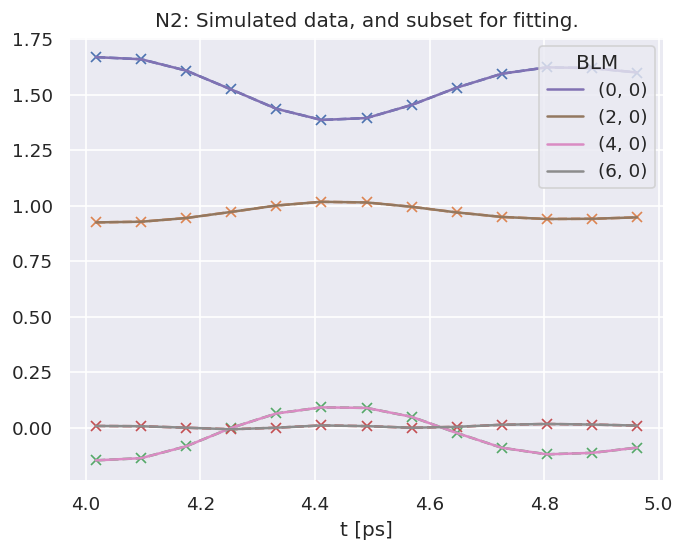
3.6.4. Time-resolved data#
In general, the datasets from a time-resolved measurement can be expressed as some form of anisotropy paramters, as outlined above. In a similar manner to the ADMs detailed in Sect. 3.5, the \(\beta_{L,M}(t)\) can be plotted directly, or expanded as distributions \(I(\epsilon,t,\theta,\phi...)\). A brief demonstration is given below, making use of the \(N_2\) dataset explored in the case study in Chpt. 8, for further details of the computational and plotting tools see Part II, and the ePSproc documentation [35] and PEMtk documentation [20].
# Configure settings for case study
# %run '../scripts/setup_notebook.py'
# Fitting setup including data generation and parameter creation
# NOTE this assumes relevant data is available in ../part2/n2fitting.
# See Part 2 for more details and data sources
fitSystem = 'N2'
dataName = 'n2fitting'
# Set datapath,
dataPath = Path(Path.cwd().parent,'part2',dataName)
# Run general config script with dataPath set above
%run "../scripts/setup_fit_case-studies_270723.py" -d {dataPath} -c {fitSystem}
Show code cell output
*** Setting up demo fitting workspace and main `data` class object...
Script: QM3 case studies
For more details see https://pemtk.readthedocs.io/en/latest/fitting/PEMtk_fitting_basic_demo_030621-full.html
To use local source code, pass the parent path to this script at run time, e.g. "setup_fit_demo ~/github"
* Loading packages...
* Loading demo matrix element data from /home/jovyan/jake-home/buildTmp/_latest_build/html/doc-source/part2/n2fitting
*** Job subset details
Key: subset
No 'job' info set for self.data[subset].
*** Job orb6 details
Key: orb6
Dir /home/jovyan/jake-home/buildTmp/_latest_build/html/doc-source/part2/n2fitting, 1 file(s).
{ 'batch': 'ePS n2, batch n2_1pu_0.1-50.1eV, orbital A2',
'event': ' N2 A-state (1piu-1)',
'orbE': -17.09691397835426,
'orbLabel': '1piu-1'}
*** Job orb5 details
Key: orb5
Dir /home/jovyan/jake-home/buildTmp/_latest_build/html/doc-source/part2/n2fitting, 1 file(s).
{ 'batch': 'ePS n2, batch n2_3sg_0.1-50.1eV, orbital A2',
'event': ' N2 X-state (3sg-1)',
'orbE': -17.34181645456815,
'orbLabel': '3sg-1'}
*** Running with default N2 settings.
* Loading demo ADM data from file /home/jovyan/jake-home/buildTmp/_latest_build/html/doc-source/part2/n2fitting/N2_ADM_VM_290816.mat...
* Subselecting data...
*** Setting for N2 case study.
Subselected from dataset 'orb5', dataType 'matE': 36 from 11016 points (0.33%)
Subselected from dataset 'pol', dataType 'pol': 1 from 3 points (33.33%)
Subselected from dataset 'ADM', dataType 'ADM': 52 from 14764 points (0.35%)
* Calculating AF-BLMs...
Running for 13 t-points
Subselected from dataset 'sim', dataType 'AFBLM': 52 from 52 points (100.00%)
*Setting up fit parameters (with constraints)...
Set 6 complex matrix elements to 12 fitting params, see self.params for details.
Auto-setting parameters.
Basis set size = 12 params. Fitting with 4 magnitudes and 3 phases floated.
*** Setup demo fitting workspace OK.
Dataset: subset, AFBLM
Dataset: sim, AFBLM
| name | value | initial value | min | max | vary | expression |
|---|---|---|---|---|---|---|
| m_PU_SG_PU_1_n1_1_1 | 1.78461575 | 1.784615753610107 | 1.0000e-04 | 5.00000000 | True | |
| m_PU_SG_PU_1_1_n1_1 | 1.78461575 | 1.784615753610107 | 1.0000e-04 | 5.00000000 | False | m_PU_SG_PU_1_n1_1_1 |
| m_PU_SG_PU_3_n1_1_1 | 0.80290495 | 0.802904951323892 | 1.0000e-04 | 5.00000000 | True | |
| m_PU_SG_PU_3_1_n1_1 | 0.80290495 | 0.802904951323892 | 1.0000e-04 | 5.00000000 | False | m_PU_SG_PU_3_n1_1_1 |
| m_SU_SG_SU_1_0_0_1 | 2.68606212 | 2.686062120382649 | 1.0000e-04 | 5.00000000 | True | |
| m_SU_SG_SU_3_0_0_1 | 1.10915311 | 1.109153108617096 | 1.0000e-04 | 5.00000000 | True | |
| p_PU_SG_PU_1_n1_1_1 | -0.86104140 | -0.8610414024232179 | -3.14159265 | 3.14159265 | False | |
| p_PU_SG_PU_1_1_n1_1 | -0.86104140 | -0.8610414024232179 | -3.14159265 | 3.14159265 | False | p_PU_SG_PU_1_n1_1_1 |
| p_PU_SG_PU_3_n1_1_1 | -3.12044446 | -3.1204444620772467 | -3.14159265 | 3.14159265 | True | |
| p_PU_SG_PU_3_1_n1_1 | -3.12044446 | -3.1204444620772467 | -3.14159265 | 3.14159265 | False | p_PU_SG_PU_3_n1_1_1 |
| p_SU_SG_SU_1_0_0_1 | 2.61122920 | 2.611229196458127 | -3.14159265 | 3.14159265 | True | |
| p_SU_SG_SU_3_0_0_1 | -0.07867828 | -0.07867827542158025 | -3.14159265 | 3.14159265 | True |
# Compute AFBLMs for all matrix elements (energies) for selected orbital
# (Note the main fitting script only computes for a single E-point.)
# Use ADMs from fitting subset
orbKey = 'orb5'
data.AFBLM(keys = orbKey, AKQS = data.data['subset']['ADM'],
selDims = {'Type':'L'}, thres=1e-2)
Calculating AF-BLMs for job key: orb5
In this case, making use of ab initio radial matrix elements, a full set of \(\beta_{L,M}(\epsilon,t)\) are computed, for the ionizing channel(s) defined (in this case as labelled by the orbKey parameter). These can be plotted vs. energy or time as line-plots or colourmaps. The Photoelectron Metrology Toolkit [5] currently has some basic routines for some specific cases, or low-level functionality from the base libraries can be used for more control.
# Default plot with Holoviews/Bokeh
# Will plot BLM(E,t) data with selectors & sliders for other dimensions
data.BLMplot(keys=orbKey, backend='hv')
BLMplot set data and plots to self.plots['BLMplot']
True
# For a full BLM(E,t) surface, the output Holoviews dataset can be used.
# See the Holoviews (https://holoviews.org) and HVplot (https://hvplot.holoviz.org) docs for more details
# Set opts to match sizes - should be able to link plots or set gridspace to handle this?
ep.plot.hvPlotters.setPlotDefaults(fSize = [750,300], imgSize = 600)
# Plot heatmap for l=2 vs. Eke and add ADM plot to layout with hvplot
daLayout = (data.plots['BLMplot']['hvDS'].select(l=[2]).to(hv.HeatMap, kdims=['t','Eke']).opts(cmap='coolwarm') +
data.data['subset']['ADM'].unstack().sel({'K':[2,4]}).squeeze().real.hvplot.line(x='t').overlay('K')).cols(1)
Show code cell content
# Glue figure for later
glue("N2BLMtDemo", daLayout)
WARNING:param.HeatMapPlot08300: Due to internal constraints, when aspect and width/height is set, the bokeh backend uses those values as frame_width/frame_height instead. This ensures the aspect is respected, but means that the plot might be slightly larger than anticipated. Set the frame_width/frame_height explicitly to suppress this warning.
Fig. 3.20 Example \(I(\epsilon,t)\) data, computed for \(N_2\) (upper panel), and the ADMs used in the calculation (lower panel).#
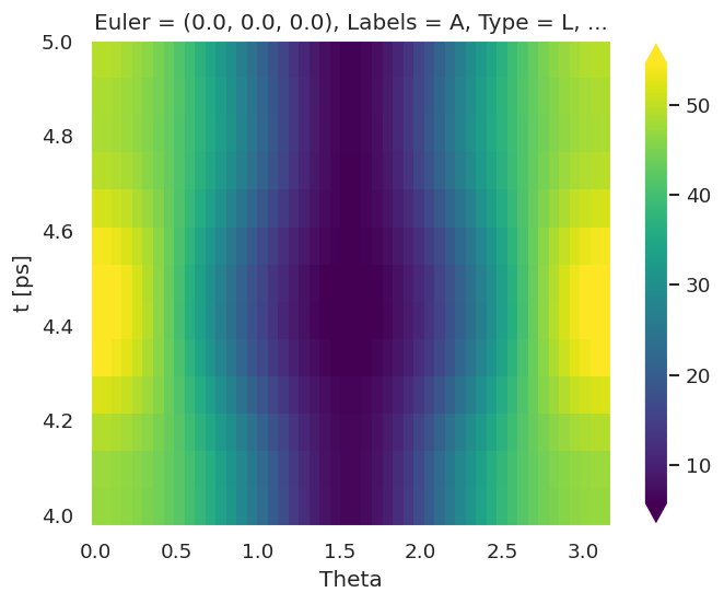
# Similarly, AFPADs can be plotted.
# Plot I(theta,t) for a single E
# %matplotlib inline
dataKey = 'subset' # Use subset data set for fitting
data.padPlot(keys = dataKey, dataType='AFBLM', selDims={'Labels':'A'},
Etype = 't', pStyle='grid', reducePhi='sum',
returnFlag = True)
Using default sph betas.
Summing over dims: set()
Plotting from self.data[subset][AFBLM], facetDims=['t', None], pType=a with backend=mpl.
Grid plot: 3sg-1, dataType: AFBLM, plotType: a
Set plot to self.data['subset']['plots']['AFBLM']['grid']
# Plot I(theta,phi) at selected (E,t)
data.padPlot(keys = dataKey, dataType='AFBLM', selDims={'Labels':'A'},
Erange=[4,5,5], Etype = 't', returnFlag = True, backend='pl')
# And GLUE for display later with caption
figObj = data.data[dataKey]['plots']['AFBLM']['polar'][0]
glue("N2AFPADsdemo", figObj)
Show code cell output
Using default sph betas.
Summing over dims: set()
Plotting from self.data[subset][AFBLM], facetDims=['t', None], pType=a with backend=pl.
Set plot to self.data['subset']['plots']['AFBLM']['polar']
Fig. 3.21 AF-PADs (\(I(\theta,\phi;\epsilon,t)\)) example for \(N_2\) at selected \((\epsilon,t)\). In this demo case the alignment and PADs are “1D”, and cylindrically symmetric.#