This page was auto-generated from a Jupyter notebook: XeF2/xef2_1.0-60.1eV_orb12_A1G.
Problems? Please raise any issues on Github.
![]()

ePSproc: xef2 wavefn run, orb 12 ioinzation (Iodine 3d, A1G/SG), 1-60eV
electronic structure input: xef2_SPKrATZP_rel_geom_v2.molden
ePS output file: xef2_1.0-60.1eV_orb12_A1G.inp.out
Web version: https://phockett.github.io/ePSdata/xef2_1.0-60.1eV/xef2_1.0-60.1eV_orb12_A1G.html
Dataset: https://zenodo.org/record/3676893
DOI (dataset): 10.5281/zenodo.3676893
Licensed under Creative Commons Attribution-NonCommercial-ShareAlike 4.0 (CC BY-NC-SA 4.0)
Job details
ePS xef2, batch xef2_1.0-60.1eV, orbital orb12_A1G
xef2 wavefn run on AntonJr, orb 12 ioinzation (Iodine 3d, A1G/SG), sph/ grid
E=1.0:2.5:60.1 (24 points)
Tue Feb 12 19:42:57 EST 2019
Set-up
Load modules
[1]:
import sys
import os
import numpy as np
import epsproc as ep

from datetime import datetime as dt
timeString = dt.now()
* pyevtk not found, VTK export not available.
* plotly not found, plotly plots not available.
Load data
[2]:
# File path only, from env var DATAFILE
# dataPath = os.getcwd()
dataFile = os.environ.get('DATAFILE', '')
[3]:
jobInfo = ep.headerFileParse(dataFile)
molInfo = ep.molInfoParse(dataFile)
*** Job info from file header.
ePS xef2, batch xef2_1.0-60.1eV, orbital orb12_A1G
xef2 wavefn run on AntonJr, orb 12 ioinzation (Iodine 3d, A1G/SG), sph/ grid
E=1.0:2.5:60.1 (24 points)
Tue Feb 12 19:42:57 EST 2019
*** Found orbitals
1 1 Ene = -1276.2548 Spin =Alpha Occup = 2.000000
2 2 Ene = -202.4761 Spin =Alpha Occup = 2.000000
3 3 Ene = -181.5792 Spin =Alpha Occup = 2.000000
4 4 Ene = -181.5770 Spin =Alpha Occup = 2.000000
5 5 Ene = -181.5770 Spin =Alpha Occup = 2.000000
6 6 Ene = -43.1198 Spin =Alpha Occup = 2.000000
7 7 Ene = -36.1973 Spin =Alpha Occup = 2.000000
8 8 Ene = -36.1881 Spin =Alpha Occup = 2.000000
9 9 Ene = -36.1881 Spin =Alpha Occup = 2.000000
10 10 Ene = -26.3038 Spin =Alpha Occup = 2.000000
11 11 Ene = -26.3038 Spin =Alpha Occup = 2.000000
12 12 Ene = -25.8711 Spin =Alpha Occup = 2.000000
13 13 Ene = -25.8673 Spin =Alpha Occup = 2.000000
14 14 Ene = -25.8673 Spin =Alpha Occup = 2.000000
15 15 Ene = -25.8578 Spin =Alpha Occup = 2.000000
16 16 Ene = -25.8578 Spin =Alpha Occup = 2.000000
17 17 Ene = -8.5562 Spin =Alpha Occup = 2.000000
18 18 Ene = -6.2727 Spin =Alpha Occup = 2.000000
19 19 Ene = -6.2547 Spin =Alpha Occup = 2.000000
20 20 Ene = -6.2547 Spin =Alpha Occup = 2.000000
21 21 Ene = -2.8143 Spin =Alpha Occup = 2.000000
22 22 Ene = -2.8032 Spin =Alpha Occup = 2.000000
23 23 Ene = -2.8032 Spin =Alpha Occup = 2.000000
24 24 Ene = -2.7810 Spin =Alpha Occup = 2.000000
25 25 Ene = -2.7810 Spin =Alpha Occup = 2.000000
26 26 Ene = -1.5681 Spin =Alpha Occup = 2.000000
27 27 Ene = -1.5619 Spin =Alpha Occup = 2.000000
28 28 Ene = -1.0877 Spin =Alpha Occup = 2.000000
29 29 Ene = -0.7372 Spin =Alpha Occup = 2.000000
30 30 Ene = -0.6738 Spin =Alpha Occup = 2.000000
31 31 Ene = -0.6738 Spin =Alpha Occup = 2.000000
32 32 Ene = -0.6426 Spin =Alpha Occup = 2.000000
33 33 Ene = -0.6426 Spin =Alpha Occup = 2.000000
34 34 Ene = -0.5518 Spin =Alpha Occup = 2.000000
35 35 Ene = -0.4994 Spin =Alpha Occup = 2.000000
36 36 Ene = -0.4994 Spin =Alpha Occup = 2.000000
*** Found atoms
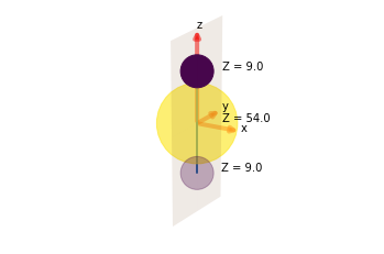
Z = 54 ZS = 54 r = 0.0000000000 0.0000000000 0.0000000000
Z = 9 ZS = 9 r = 0.0000000000 0.0000000000 -1.9373220000
Z = 9 ZS = 9 r = 0.0000000000 0.0000000000 1.9373220000
[4]:
# Scan file(s) for various data types...

# For dir scan
# dataXS = ep.readMatEle(fileBase = dataPath, recordType = 'CrossSection')
# dataMatE = ep.readMatEle(fileBase = dataPath, recordType = 'DumpIdy')

# For single file
dataXS = ep.readMatEle(fileIn = dataFile, recordType = 'CrossSection')
dataMatE = ep.readMatEle(fileIn = dataFile, recordType = 'DumpIdy')
*** ePSproc readMatEle(): scanning files for CrossSection segments.

*** Scanning file(s)
['/mnt/femtobackSSHFS/FemtoShare/Results/ePolyScat_stuff/xef2/xef2_1.0-60.1eV/xef2_1.0-60.1eV_orb12_A1G.inp.out']

*** Reading ePS output file:  /mnt/femtobackSSHFS/FemtoShare/Results/ePolyScat_stuff/xef2/xef2_1.0-60.1eV/xef2_1.0-60.1eV_orb12_A1G.inp.out
Expecting 24 energy points.
Expecting 2 symmetries.
Scanning CrossSection segments.
Expecting 3 CrossSection segments.
Found 3 CrossSection segments (sets of results).
Processed 3 sets of CrossSection file segments, (0 blank)
*** ePSproc readMatEle(): scanning files for DumpIdy segments.

*** Scanning file(s)
['/mnt/femtobackSSHFS/FemtoShare/Results/ePolyScat_stuff/xef2/xef2_1.0-60.1eV/xef2_1.0-60.1eV_orb12_A1G.inp.out']

*** Reading ePS output file:  /mnt/femtobackSSHFS/FemtoShare/Results/ePolyScat_stuff/xef2/xef2_1.0-60.1eV/xef2_1.0-60.1eV_orb12_A1G.inp.out
Expecting 24 energy points.
Expecting 2 symmetries.
Scanning CrossSection segments.
Expecting 48 DumpIdy segments.
Found 48 dumpIdy segments (sets of matrix elements).

Processing segments to Xarrays...
Processed 48 sets of DumpIdy file segments, (0 blank)
Job & molecule info
[5]:
ep.jobSummary(jobInfo, molInfo);
*** Job summary data
 ePS xef2, batch xef2_1.0-60.1eV, orbital orb12_A1G
 xef2 wavefn run on AntonJr, orb 12 ioinzation (Iodine 3d, A1G/SG), sph/ grid
 E=1.0:2.5:60.1 (24 points)
 Tue Feb 12 19:42:57 EST 2019

Electronic structure input: '/home/paul/ePS_stuff/xef2/electronic_structure/xef2_SPKrATZP_rel_geom_v2.molden'
Initial state occ:               [2 2 2 4 2 2 4 2 2 2 4 4 2 2 4 2 4 4 2 2 2 2 4 4 2 4]
Final state occ:                 [2 2 2 4 2 2 4 2 2 1 4 4 2 2 4 2 4 4 2 2 2 2 4 4 2 4]
IPot (input vertical IP, eV):            12.35

*** Additional orbital info (SymProd)
Ionizing orb:                    [0 0 0 0 0 0 0 0 0 1 0 0 0 0 0 0 0 0 0 0 0 0 0 0 0 0]
Ionizing orb sym:                ['SG']
Orb energy (eV):                 [-703.98848886]
Orb energy (H):                  [-25.8711]
Orb energy (cm^-1):              [-5678050.13578627]
Threshold wavelength (nm):       1.7611679645049914

*** Warning: some orbital convergences outside single-center expansion convergence tolerance (0.01):
[[10.          0.81998167]
 [11.          0.80599244]
 [26.          0.9860914 ]
 [27.          0.98404896]]

*** Molecular structure
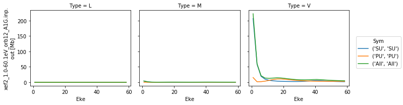
1-photon ePS Cross-Sections
Plot 1-photon cross-sections and \(beta_2\) parameters (for an unaligned ensemble) from ePS calculations. These are taken directly from the ePS output file, CrossSection segments. See the ePS manual, ``GetCro` command, for further details <https://www.chem.tamu.edu/rgroup/lucchese/ePolyScat.E3.manual/GetCro.html>`__.
Cross-sections by symmetry & type
Types correspond to:
‘L’: length gauge results.
‘V’: velocity gauge results.
‘M’: mixed gauge results.
Symmetries correspond to allowed ionizing transitions for the molecular point group (IRs typically corresponding to (x,y,z) polarization geometries), see the ePS manual for a list of symmetries. Symmetry All corresponds to the sum over all allowed sets of symmetries.
Cross-section units are MBarn.
[6]:
# Plot cross sections using Xarray functionality
# Set here to plot per file - should add some logic to combine files.
for data in dataXS:
    daPlot = data.sel(XC='SIGMA')
    daPlot.plot.line(x='Eke', col='Type')
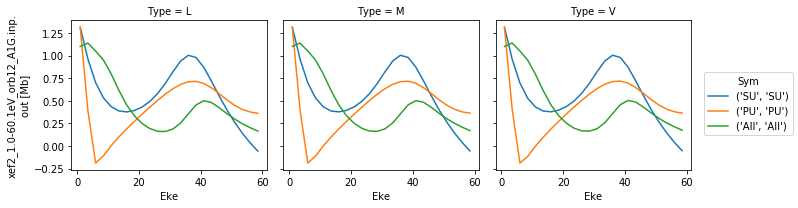
\(\beta_{2}\) by symmetry & type
Types & symmetries as per cross-sections. Normalized \(\beta_{2}\) paramters, dimensionless.
[7]:
# Repeat for betas
for data in dataXS:
    daPlot = data.sel(XC='BETA')
    daPlot.plot.line(x='Eke', col='Type')
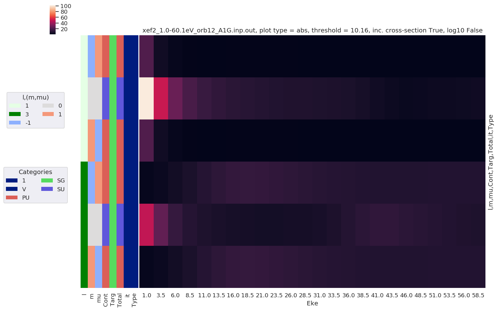
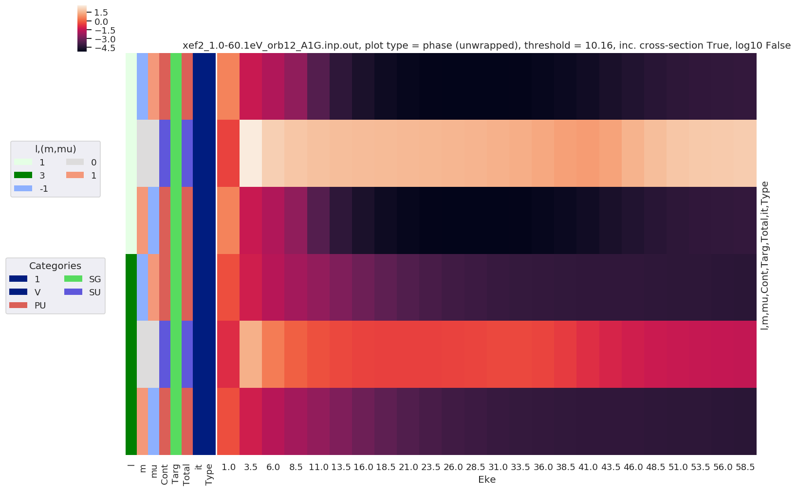
Dipole matrix elements
For 1-photon ionization. These are taken directly from ePS DumpIdy segments. See the ePS manual, ``DumpIdy` command, for further details <https://www.chem.tamu.edu/rgroup/lucchese/ePolyScat.E3.manual/DumpIdy.html>`__.
[8]:
# Set threshold for significance, only matrix elements with abs values > thres % will be plotted
thres = 0.1
[9]:
# Plot for each fie
for data in dataMatE:
    # Plot with sensible defaults - all dims with lmPlot()

    # Plot only values > theshold
    daPlot, daPlotpd, legendList, gFig = ep.lmPlot(data, thres = thres, thresType = 'pc', figsize = (15,10))

    # Plot phases, with unwrap
    daPlot, daPlotpd, legendList, gFig = ep.lmPlot(data, thres = thres, thresType = 'pc', figsize = (15,10), pType='phaseUW')
/home/paul/anaconda3/envs/ePSproc-v1.2/lib/python3.7/site-packages/xarray/core/nputils.py:223: RuntimeWarning: All-NaN slice encountered
  result = getattr(npmodule, name)(values, axis=axis, **kwargs)
Plotting data xef2_1.0-60.1eV_orb12_A1G.inp.out, pType=a, thres=10.1581107134, with Seaborn
/home/paul/anaconda3/envs/ePSproc-v1.2/lib/python3.7/site-packages/xarray/core/nputils.py:223: RuntimeWarning: All-NaN slice encountered
  result = getattr(npmodule, name)(values, axis=axis, **kwargs)
/home/paul/anaconda3/envs/ePSproc-v1.2/lib/python3.7/site-packages/numpy/lib/function_base.py:1520: RuntimeWarning: invalid value encountered in greater
  _nx.copyto(ddmod, pi, where=(ddmod == -pi) & (dd > 0))
/home/paul/anaconda3/envs/ePSproc-v1.2/lib/python3.7/site-packages/numpy/lib/function_base.py:1522: RuntimeWarning: invalid value encountered in less
  _nx.copyto(ph_correct, 0, where=abs(dd) < discont)
Plotting data xef2_1.0-60.1eV_orb12_A1G.inp.out, pType=phaseUW, thres=10.1581107134, with Seaborn
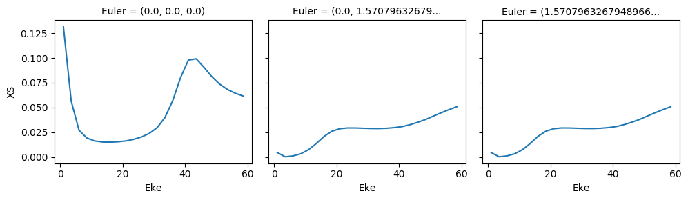
MFPADs
Calculated MF \(\beta\) parameters, using ePS dipole matrix elements. These are calculated by ep.mfblm(), as a function of energy and polarization geometry. See the ePSproc docs on ``ep.mfblm()` <https://epsproc.readthedocs.io/en/latest/modules/epsproc.MFBLM.html>`__ for further details, and this demo notebook.
[10]:
# Set pol geoms - these correspond to (z,x,y) in molecular frame (relative to principle/symmetry axis)
eAngs = ep.setPolGeoms()
[11]:
# Drop threshold for MF calcs
thres = 1e-3
# Calculate for each fie & pol geom
# TODO - file logic, and parallelize
BLM = []
for data in dataMatE:
    BLM.append(ep.mfblmEuler(data, selDims = {'Type':'L'}, eAngs = eAngs, thres = thres,
                             SFflag = True, verbose = 0))  # Run for all Eke, selected gauge only
[12]:
# Save BLM data - defaults to working dir and 'ep_timestamp' file
# TODO - testing for array/multiple file case
for data in BLM:
    fileName = dataFile + '_BLM-L_' + timeString.strftime('%Y-%m-%d_%H-%M-%S')
    ep.writeXarray(data, fileName = fileName)
['Written to h5netcdf format', '/mnt/femtobackSSHFS/FemtoShare/Results/ePolyScat_stuff/xef2/xef2_1.0-60.1eV/xef2_1.0-60.1eV_orb12_A1G.inp.out_BLM-L_2020-02-13_16-07-43.nc']
/home/paul/anaconda3/envs/ePSproc-v1.2/lib/python3.7/site-packages/h5netcdf/core.py:481: H5pyDeprecationWarning: other_ds.dims.create_scale(ds, name) is deprecated. Use ds.make_scale(name) instead.
  h5ds.dims.create_scale(h5ds, scale_name)
[13]:
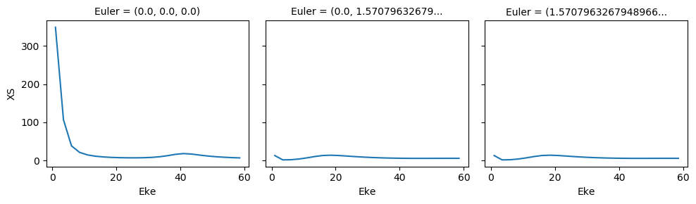
# Normalize and plot results
for BLMplot in BLM:
# Plot unnormalized B00 only, real part
# This is/should be in units of MBarn (TBC).
# BLMplot.where(np.abs(BLMplot) > thres, drop = True).real.squeeze().sel({'l':0, 'm':0}).plot.line(x='Eke', col='Euler');
BLMplot.XS.real.squeeze().plot.line(x='Eke', col='Euler');
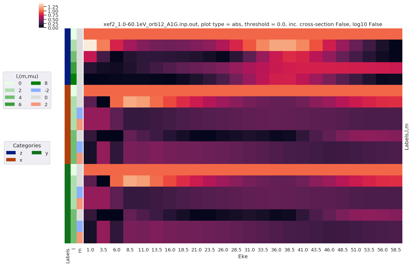
# Plot values normalised by B00 - now set in calculation function
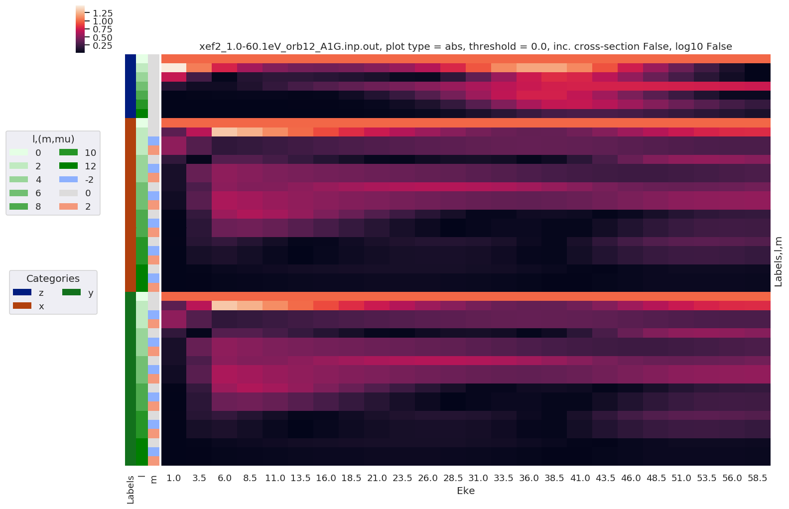
# Plot results with lmPlot(), ordering by Euler sets
# Version with (semi-manual) Euler grouping
daPlot, daPlotpd, legendList, gFig = ep.lmPlot(BLMplot.swap_dims({'Euler':'Labels'}), SFflag = False, eulerGroup = True,
thresType = 'pc', thres = thres,
plotDims = ('Labels','l','m'),
figsize = (15,10))
Plotting data xef2_1.0-60.1eV_orb12_A1G.inp.out, pType=a, thres=0.001468340773845271, with Seaborn
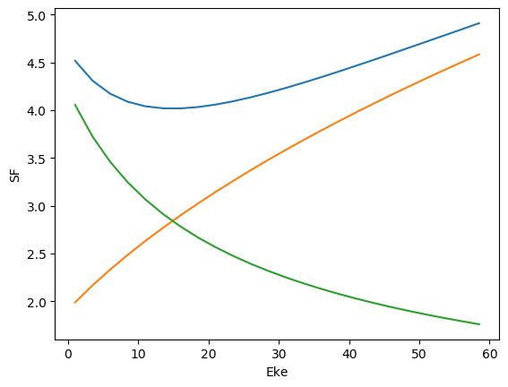
Error & consistency checks
[14]:
# Check SF values
for data in dataMatE:
    # Plot values, single plot
    data.SF.pipe(np.abs).plot.line(x='Eke')
    data.SF.real.plot.line(x='Eke')
    data.SF.imag.plot.line(x='Eke')

    # Plot values, facet plot
#     data.SF.pipe(np.abs).plot.line(x='Eke', col='Sym')
[15]:
# Compare calculated BLMs for L and V types (dafault above for L)

# Calculate for each fie & pol geom, and compare.
BLMv = []
BLMdiff = []
for n, data in enumerate(dataMatE):
    BLMv.append(ep.mfblmEuler(data, selDims = {'Type':'V'}, eAngs = eAngs, thres = thres,
                             SFflag = True, verbose = 0))  # Run for all Eke, selected gauge only

    BLMdiff.append(BLM[n] - BLMv[n])
    BLMdiff[n]['dXS'] = BLM[n].XS - BLMv[n].XS  # Set XS too, dropped in calc above

    BLMdiff[n].attrs['dataType'] = 'matE'
[16]:
# Save BLM data - defaults to working dir and 'ep_timestamp' file
# TODO - testing for array/multiple file case
for data in BLMv:
    fileName = dataFile + '_BLM-V_' + timeString.strftime('%Y-%m-%d_%H-%M-%S')
    ep.writeXarray(data, fileName = fileName)
['Written to h5netcdf format', '/mnt/femtobackSSHFS/FemtoShare/Results/ePolyScat_stuff/xef2/xef2_1.0-60.1eV/xef2_1.0-60.1eV_orb12_A1G.inp.out_BLM-V_2020-02-13_16-07-43.nc']
/home/paul/anaconda3/envs/ePSproc-v1.2/lib/python3.7/site-packages/h5netcdf/core.py:481: H5pyDeprecationWarning: other_ds.dims.create_scale(ds, name) is deprecated. Use ds.make_scale(name) instead.
  h5ds.dims.create_scale(h5ds, scale_name)
[17]:
# Normalize and plot results
for BLMplot in BLMv:
    # Plot unnormalized B00 only, real part
    # This is/should be in units of MBarn (TBC).
#     BLMplot.where(np.abs(BLMplot) > thres, drop = True).real.squeeze().sel({'l':0, 'm':0}).plot.line(x='Eke', col='Euler');
    BLMplot.XS.real.squeeze().plot.line(x='Eke', col='Euler');

    # Plot values normalised by B00 - now set in calculation function
    # Plot results with lmPlot(), ordering by Euler sets
    # Version with (semi-manual) Euler grouping
    daPlot, daPlotpd, legendList, gFig = ep.lmPlot(BLMplot.swap_dims({'Euler':'Labels'}), SFflag = False, eulerGroup = True,
                                                   thresType = 'pc', thres = thres,
                                                   plotDims = ('Labels','l','m'),
                                                   figsize = (15,10))
Plotting data xef2_1.0-60.1eV_orb12_A1G.inp.out, pType=a, thres=0.0014690955811964875, with Seaborn
[18]:
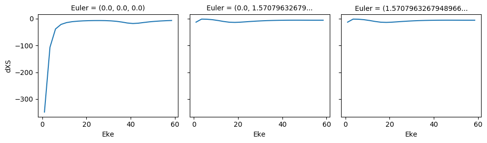
# Difference between 'L' and 'V' results
# NOTE - this currently drops XS
print('Differences, L vs. V gauge BLMs')
for BLMplot in BLMdiff:
maxDiff = BLMplot.max()
print(f'Max difference in BLMs (L-V): {0}', maxDiff.data)
if np.abs(maxDiff) > thres:
# Plot B00 only, real part
# BLMplot.where(np.abs(BLMplot) > thres, drop = True).real.squeeze().sel({'l':0, 'm':0}).plot.line(x='Eke', col='Euler');
BLMplot.dXS.real.squeeze().plot.line(x='Eke', col='Euler');
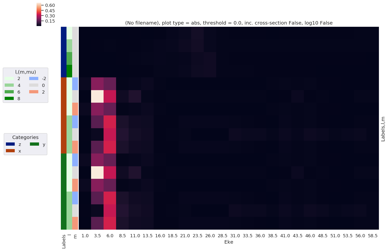
# Plot values normalised by B00 - now set in calculation function
# Plot results with lmPlot(), ordering by Euler sets
# Version with (semi-manual) Euler grouping
daPlot, daPlotpd, legendList, gFig = ep.lmPlot(BLMplot.swap_dims({'Euler':'Labels'}), SFflag = False, eulerGroup = True,
thresType = 'pc', thres = thres,
plotDims = ('Labels','l','m'),
figsize = (15,10))
Differences, L vs. V gauge BLMs
Max difference in BLMs (L-V): 0 (0.34692345160788+8.725762238127286e-17j)
Plotting data (No filename), pType=a, thres=0.00034692345160788, with Seaborn
[19]:
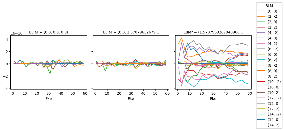
# Check imaginary components - should be around machine tolerance.
print('Machine tolerance: ', np.finfo(float).eps)
for BLMplot in BLM:
    maxImag = BLMplot.imag.max()
    print(f'Max imaginary value: {0}', maxImag.data)

#     BLMplot.where(np.abs(BLMplot) > thres, drop = True).imag.squeeze().plot.line(x='Eke', col='Euler');

    BLMplot = ep.matEleSelector(BLMplot, thres=thres, dims = 'Eke')
    BLMplot.imag.squeeze().plot.line(x='Eke', col='Euler');
Machine tolerance:  2.220446049250313e-16
Max imaginary value: 0 4.1933287884051097e-16
Version info
Original job details
[20]:
print(jobInfo['ePolyScat'][0])
print('Run: ' + jobInfo['Starting'][0].split('at')[1])
ePolyScat Version E3
Run:  2019-02-12  20:54:33.594 (GMT -0500)
ePSproc details
[21]:
templateVersion = '0.0.6'
templateDate = '12/01/20'
[22]:
%load_ext version_information
[23]:
%version_information epsproc, xarray
[23]:
| Software | Version |
|---|---|
| Python | 3.7.5 64bit [GCC 7.3.0] |
| IPython | 7.9.0 |
| OS | Linux 5.0.0 36 generic x86_64 with debian buster sid |
| epsproc | 1.2.4 |
| xarray | 0.14.0 |
| Thu Feb 13 16:10:52 2020 EST | |
[24]:
print('Run: {}'.format(timeString.strftime('%Y-%m-%d_%H-%M-%S')))
host = !hostname
print('Host: {}'.format(host[0]))
Run: 2020-02-13_16-07-43
Host: jake
Cite this dataset
Hockett, Paul (2019). ePSproc: xef2 wavefn run, orb 12 ioinzation (Iodine 3d, A1G/SG), 1-60eV. Dataset on Zenodo. DOI: 10.5281/zenodo.3676893. URL: https://phockett.github.io/ePSdata/xef2_1.0-60.1eV/xef2_1.0-60.1eV_orb12_A1G.html
Bibtex:
@data{xef2 wavefn run, orb 12 ioinzation (Iodine 3d, A1G/SG), 1-60eV,
    title = {ePSproc: xef2 wavefn run, orb 12 ioinzation (Iodine 3d, A1G/SG), 1-60eV}
    author = {Hockett, Paul},
    doi = {10.5281/zenodo.3676893},
    publisher = {Zenodo},
    year = {2019},
    url = {https://phockett.github.io/ePSdata/xef2_1.0-60.1eV/xef2_1.0-60.1eV_orb12_A1G.html}
  }
See citation notes on ePSdata for further details.
![]()