3.2. Advanced fitting for hyperfine beat (stage 1 bootstrap)#
For advanced fitting, try a stage 1 style bootstrap. In this case, options are:
“basic” ignore the photoionization dynamics and just try fitting the beat to the \(l=4\), ROI=0 case, since it is already pretty close and may be assumed to be directly mapped here. See Basic fitting for hyperfine beat (stage 1 bootstrap).
“advanced” set (arbitrary) parameters per final state for the probe, and fit these plus the hyperfine beat model parameters. This should allow for a match to a single set of hyperfine parameters for all observables, and fulfil the stage 1 bootstrap criteria. (This page.)
From prior work and data:
Forbes, R. et al. (2018) ‘Quantum-beat photoelectron-imaging spectroscopy of Xe in the VUV’, Physical Review A, 97(6), p. 063417. Available at: https://doi.org/10.1103/PhysRevA.97.063417. arXiv: http://arxiv.org/abs/1803.01081, Authorea (original HTML version): https://doi.org/10.22541/au.156045380.07795038
Data (OSF): https://osf.io/ds8mk/
Quantum Metrology with Photoelectrons (Github repo), particularly the Alignment 3 notebook. Functions from this notebook have been incorporated in the current project, under
qbanalysis.hyperfine.
3.2.1. Advanced model & fitting methodology#
3.2.1.1. Model improvements#
In order to more fully describe the data, make the following additions to the basic model:
Allow for signal decay with exponential decay and lifetimes per isotope. This can be added to the hyperfine wavepacket ((2.1)) as:
Where \(\tau_I\) is the lifetime for each isotope/nuclear spin state.
Add a phenomenological ionization model. In this case, simply allow for a magnitude and offset per channel (i.e. per \(l\), \(ROI\) in the dataset). In this case, the signal per channel can be described as the product of the wavepacket and ionization model:
In this model the amplitudes \(A\) and offsets \(O\) can be +ve or -ve, but no other phase terms are included, and they are assumed to be the same for each isotope (but not ionization channel). Note that the underlying wavepacket is effectively global, aside from the decay constants, as indicated above.
3.2.1.2. Fitting changes#
For handling larger models and fitting, lmfit can be used. This provides a method for setting and addressing parameters by name (with class and dictionary syntax), and is therefore easier to use and debug as compared the the base Scipy routines (at the cost of a slightly more elaborate setup and configuration). Note, however, that Scipy routines are still used on the backend, but lmfit provides a convenient wrapper and ancillary functionality.
3.2.2. Setup fitting model#
Follow the modelling notebook (Hyperfine beat and (electronic) alignment modelling), but wrap functions for fitting, plus updates to use advanced model + lmfit.
New functions are in qbanalysis.adv_fitting.py.
3.2.2.1. Imports#
# Load packages
# Main functions used herein from qbanalysis.hyperfine
from qbanalysis.hyperfine import *
import numpy as np
from epsproc.sphCalc import setBLMs

from pathlib import Path

dataPath = Path('/tmp/xe_analysis')
# dataTypes = ['BLMall', 'BLMerr', 'BLMerrCycle']   # Read these types, should just do dir scan here.

# # Read from HDF5/NetCDF files
# # TO FIX: this should be identical to loadFinalDataset(dataPath), but gives slightly different plots - possibly complex/real/abs confusion?
# dataDict = {}
# for item in dataTypes:
#     dataDict[item] = IO.readXarray(fileName=f'Xe_dataset_{item}.nc', filePath=dataPath.as_posix()).real
#     dataDict[item].name = item

# Read from raw data files
from qbanalysis.dataset import loadFinalDataset
dataDict = loadFinalDataset(dataPath)

# Use Pandas and load Xe local data (ODS)
# These values were detemermined from the experimental data as detailed in ref. [4].
from qbanalysis.dataset import loadXeProps
xeProps = loadXeProps()
2025-06-03 16:51:24.394 | INFO | qbanalysis.config:<module>:11 - PROJ_ROOT path is: /home/runner/work/Quantum-Beat_Photoelectron-Imaging_Spectroscopy_of_Xe_in_the_VUV/Quantum-Beat_Photoelectron-Imaging_Spectroscopy_of_Xe_in_the_VUV
* sparse not found, sparse matrix forms not available.
* natsort not found, some sorting functions not available.
* Setting plotter defaults with epsproc.basicPlotters.setPlotters(). Run directly to modify, or change options in local env.
* Set Holoviews with bokeh.
* pyevtk not found, VTK export not available.
* pyshtools not found, SHtools functions not available. If required, run "pip install pyshtools" or "conda install -c conda-forge pyshtools" to install.
2025-06-03 16:51:44.983 | INFO     | qbanalysis.hyperfine:<module>:31 - Using uncertainties modules, Sympy maths functions will be forced to float outputs.
2025-06-03 16:51:45.058 | INFO     | qbanalysis.dataset:loadDataset:268 - Loaded data cpBasex_results_cycleSummed_rot90_quad1_ROI_results_with_FT_NFFT1024_hanningWindow_270717.mat.
2025-06-03 16:51:45.108 | INFO     | qbanalysis.dataset:loadDataset:268 - Loaded data cpBasex_results_allCycles_ROIs_with_FTs_NFFT1024_hanningWindow_270717.mat.
2025-06-03 16:51:45.434 | INFO | qbanalysis.dataset:loadFinalDataset:244 - Processed data to Xarray OK.
2025-06-03 16:51:45.462 | INFO | qbanalysis.dataset:loadXeProps:71 - Loaded Xe data from /home/runner/work/Quantum-Beat_Photoelectron-Imaging_Spectroscopy_of_Xe_in_the_VUV/Quantum-Beat_Photoelectron-Imaging_Spectroscopy_of_Xe_in_the_VUV/dataLocal/Xe_data_table_fixedFractions.ods.
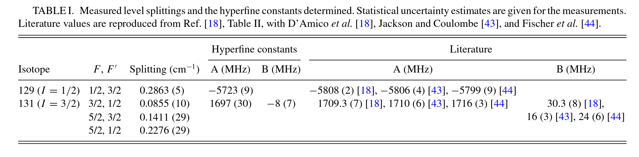
**Xe measured level splittings and the hyperfine constants.**
Statistical uncertainty estimates are given for the measurements. (See manuscript for details).
/opt/hostedtoolcache/Python/3.10.11/x64/lib/python3.10/site-packages/xarray/core/concat.py:500: FutureWarning: unique with argument that is not not a Series, Index, ExtensionArray, or np.ndarray is deprecated and will raise in a future version.
  common_dims = tuple(pd.unique([d for v in vars for d in v.dims]))
/home/runner/work/Quantum-Beat_Photoelectron-Imaging_Spectroscopy_of_Xe_in_the_VUV/Quantum-Beat_Photoelectron-Imaging_Spectroscopy_of_Xe_in_the_VUV/qbanalysis/dataset.py:82: FutureWarning: DataFrame.applymap has been deprecated. Use DataFrame.map instead.
  tidied = rawXeHyperfineResults.applymap(lambda x: x.replace(' ','') if isinstance(x, str) else x)
/home/runner/work/Quantum-Beat_Photoelectron-Imaging_Spectroscopy_of_Xe_in_the_VUV/Quantum-Beat_Photoelectron-Imaging_Spectroscopy_of_Xe_in_the_VUV/qbanalysis/dataset.py:87: FutureWarning: DataFrame.applymap has been deprecated. Use DataFrame.map instead.
  tidied[uList] = tidied[uList].applymap(lambda x: ufloat_fromstr(x))  # OK
| A/MHz | B/MHz | Splitting/cm−1 | ||||
|---|---|---|---|---|---|---|
| Isotope | I | F | F′ | |||
| 129 | 0.5 | 0.5 | 1.5 | -5723+/-9 | nan+/-nan | 0.2863+/-0.0005 |
| 131 | 1.5 | 1.5 | 0.5 | 1697+/-30 | -8+/-7 | 0.0855+/-0.0010 |
| 2.5 | 1.5 | 1697+/-30 | -8+/-7 | 0.1411+/-0.0029 | ||
| 0.5 | 1697+/-30 | -8+/-7 | 0.2276+/-0.0029 |
# v2 pkg
from qbanalysis.adv_fitting import *
2025-06-03 16:51:45.507 | INFO     | qbanalysis.basic_fitting:<module>:21 - Using uncertainties modules, Sympy maths functions will be forced to float outputs.
2025-06-03 16:51:45.507 | INFO     | qbanalysis.adv_fitting:<module>:29 - Using uncertainties modules, Sympy maths functions will be forced to float outputs.
Show code cell content
# Hide future warnings from Xarray concat for fitting on some platforms
import warnings
# warnings.filterwarnings('ignore')  # ALL WARNINGS
# warnings.filterwarnings('ignore', category=DeprecationWarning)
warnings.filterwarnings('ignore', category=FutureWarning)
3.2.2.2. Init parameters#
Here the defaults can be used initially, and later modified as desired.
Here:
the basic model parameters for the level splittings are
s0, s1...,the lifetimes per isotope are
tau129andtau131\(A_{l,I}\), \(O_{l,I}\) are denoted
l<N>_<param>_<ROI>, for \(N=2,4\),<param>=amp,offand<ROI>=0,1to match the channels in the experimental data.
# Create model parameters
params = initParams(xeProps)

# Display default repr
params
| name | value | initial value | min | max | vary |
|---|---|---|---|---|---|
| s0 | 0.28630000 | 0.2863 | 0.00000000 | 1.00000000 | True |
| s1 | 0.08550000 | 0.0855 | 0.00000000 | 1.00000000 | True |
| s2 | 0.14110000 | 0.1411 | 0.00000000 | 1.00000000 | True |
| s3 | 0.22760000 | 0.2276 | 0.00000000 | 1.00000000 | True |
| tau129 | 5000.00000 | 5000 | 0.00000000 | 200000.000 | True |
| tau131 | 5000.00000 | 5000 | 0.00000000 | 200000.000 | True |
| l2_amp_0 | 1.68320932 | 1.683209316462884 | -10.0000000 | 10.0000000 | True |
| l4_amp_0 | -5.20756982 | -5.207569817771384 | -10.0000000 | 10.0000000 | True |
| l2_offset_0 | -3.56035953 | -3.5603595302689772 | -10.0000000 | 10.0000000 | True |
| l4_offset_0 | 3.41569948 | 3.415699478887129 | -10.0000000 | 10.0000000 | True |
| l2_amp_1 | 4.03092228 | 4.030922278904169 | -10.0000000 | 10.0000000 | True |
| l4_amp_1 | -2.01608983 | -2.0160898283183615 | -10.0000000 | 10.0000000 | True |
| l2_offset_1 | -3.45381677 | -3.453816769281959 | -10.0000000 | 10.0000000 | True |
| l4_offset_1 | -3.34121708 | -3.3412170818021902 | -10.0000000 | 10.0000000 | True |
# Parameter values can be modified with params.set()
params.set(l2_amp_0=1)

# Or use dict syntax to chnage other properties
params.set(s1={'max':0.5})
params.set(s2={'vary':False})  # Skip this parameter as it is not actually used


# Properties can be checked by name or .get
print(params['l2_amp_0'])
print(params.get('s1'))
<Parameter 'l2_amp_0', value=1, bounds=[-10:10]>
<Parameter 's1', value=array(0.0855), bounds=[0:0.5]>
3.2.3. Set data and test model#
# Set data for l=2,4, and uncertainties
dataIn = dataDict['BLMall'].unstack().sel({'l':[2,4]}).copy()
dataUn = dataDict['BLMerr'].unstack().sel({'l':[2,4]}).copy()  # Main data has uncertainties separately currently
# Compute advanced model...
calcDict = calcAdvFitModel(params, xePropsFit=xeProps, dataDict=dataDict)

# Note this returns various stages of the calculation in the output dict
calcDict.keys()
dict_keys(['xData', 'xePropsFit', 'dataDict', 'trange', 'fitFlag', 'returnType', 'modelDict', 'modelDictSum', 'modelDA', 'modelSum', 'dataIn', 'modelIn', 'res', 'iso', 'dataCol', 'decay', 'ionization'])
# Plot original (basic) model, and model with decay
plotHyperfineModel(calcDict['modelDA']) * plotHyperfineModel(calcDict['decay'])
# Plot ionization model - this now has channels to match experimental case (l,ROI)
plotHyperfineModel(calcDict['ionization'].squeeze(),overlay=['l'])
3.2.4. Fitting with the advanced model#
Here use qbanalysis.adv_fitting.calcAdvlmfit() - this wraps the above model + residual calculations for lmfit.
mini = lmfit.Minimizer(calcAdvlmfit, params, fcn_kws={'xePropsFit':xeProps, 'dataDict':dataDict})
result = mini.minimize()
/opt/hostedtoolcache/Python/3.10.11/x64/lib/python3.10/site-packages/uncertainties/core.py:1024: UserWarning: Using UFloat objects with std_dev==0 may give unexpected results.
  warn("Using UFloat objects with std_dev==0 may give unexpected results.")
# Check final output and plot vs. data
# from qbanalysis.plots import plotFinalDatasetBLMt
# plotOpts = {'width':800}
# calcDict = calcAdvFitModel(out.params, xePropsFit=xeProps, dataDict=dataDict)
# plotHyperfineModel(calcDict['ionization'],overlay=['ROI']) * plotFinalDatasetBLMt(**dataDict, **plotOpts)


# PLOT TESTING...
# TODO: add labels and fix ledgend in layout
from qbanalysis.plots import plotFinalDatasetBLMt
plotOpts = {'width':800}
calcDict = calcAdvFitModel(result.params, xePropsFit=xeProps, dataDict=dataDict)
# plotHyperfineModel(calcDict['ionization'],overlay=['ROI']).layout('l')

# To fix layout issues, treat l separately...
l2 = (plotFinalDatasetBLMt(**dataDict) * plotHyperfineModel(calcDict['ionization'],overlay=['ROI'])).select(l=2)
l4 = (plotFinalDatasetBLMt(**dataDict) * plotHyperfineModel(calcDict['ionization'],overlay=['ROI'])).select(l=4)

(l2.overlay('l').opts(title="l2", **plotOpts) + l4.overlay('l').opts(title="l4", **plotOpts)).cols(1)
# Check final residuals
res, dataDS, modelDS = residualAdv(calcDict['ionization'].squeeze(), dataIn.squeeze(), dataUn = dataUn)
plotHyperfineModel(res,overlay=['l'], **plotOpts)
# Final fit parameters
# result.params.pretty_print()
result.params
| name | value | standard error | relative error | initial value | min | max | vary |
|---|---|---|---|---|---|---|---|
| s0 | 0.29113547 | 2.5714e-04 | (0.09%) | 0.2863 | 0.00000000 | 1.00000000 | True |
| s1 | 0.08509328 | 8.9181e-04 | (1.05%) | 0.0855 | 0.00000000 | 0.50000000 | True |
| s2 | 0.14110000 | 0.00000000 | (0.00%) | 0.1411 | 0.00000000 | 1.00000000 | False |
| s3 | 0.23093377 | 7.1831e-04 | (0.31%) | 0.2276 | 0.00000000 | 1.00000000 | True |
| tau129 | 3389.28714 | 928.302541 | (27.39%) | 5000 | 0.00000000 | 200000.000 | True |
| tau131 | 3765.62509 | 1321.56285 | (35.10%) | 5000 | 0.00000000 | 200000.000 | True |
| l2_amp_0 | 1.94104718 | 0.14739955 | (7.59%) | 1 | -10.0000000 | 10.0000000 | True |
| l4_amp_0 | 1.87625265 | 0.07115181 | (3.79%) | -5.207569817771384 | -10.0000000 | 10.0000000 | True |
| l2_offset_0 | 0.47571690 | 0.00759597 | (1.60%) | -3.5603595302689772 | -10.0000000 | 10.0000000 | True |
| l4_offset_0 | -0.01934225 | 0.00168126 | (8.69%) | 3.415699478887129 | -10.0000000 | 10.0000000 | True |
| l2_amp_1 | -1.80550596 | 0.24973865 | (13.83%) | 4.030922278904169 | -10.0000000 | 10.0000000 | True |
| l4_amp_1 | -1.91628164 | 0.12548802 | (6.55%) | -2.0160898283183615 | -10.0000000 | 10.0000000 | True |
| l2_offset_1 | 0.57907054 | 0.01081064 | (1.87%) | -3.453816769281959 | -10.0000000 | 10.0000000 | True |
| l4_offset_1 | 0.15870695 | 0.00481503 | (3.03%) | -3.3412170818021902 | -10.0000000 | 10.0000000 | True |
Of note here is that the uncertainties are generally quite small, with the exception of the \(\tau\) parameters. In the current case - fitting only \(\beta>0\) - these parameters should only be relevant/necessary if (a) there is significant signal decay such that S/N becomes an issue (as in the \((L=2,ROI=1)\) channel), (b) there is a loss in coherence of the wavepacket. This is becuase the data is already normalised by yield, so any population or signal decay is removed. Here it seems that (b) is likely to be long, on the order of 4 ns, with a large uncertainty, which should be comparable to the state lifetimes.
TODO: try basic fitting for yields (\(L=0\)) to chek \(\tau\) values, although there are likely to be other issues there.
3.2.5. Check hyperfine A, B params from the updated model#
from qbanalysis.basic_fitting import extractABParams
xePropsFit =extractABParams(calcDict['xePropsFit'])
xePropsFit.style.set_caption("Updated results")
/opt/hostedtoolcache/Python/3.10.11/x64/lib/python3.10/site-packages/scipy/optimize/_lsq/least_squares.py:825: UserWarning: Setting `gtol` below the machine epsilon (2.22e-16) effectively disables the corresponding termination condition.
  ftol, xtol, gtol = check_tolerance(ftol, xtol, gtol, method)
`gtol` termination condition is satisfied.
Function evaluations 16, initial cost 8.6538e-07, final cost 1.2884e-24, first-order optimality 9.83e-19.
| A/MHz | B/MHz | Splitting/cm−1 | label | ||||
|---|---|---|---|---|---|---|---|
| Isotope | I | F | F′ | ||||
| 129 | 0.500000 | 0.500000 | 1.500000 | -5818.681222 | nan+/-nan | 0.291135 | s0 |
| 131 | 1.500000 | 1.500000 | 0.500000 | 1740.852909 | 40.154531 | 0.085093 | s1 |
| 2.500000 | 1.500000 | 1740.852909 | 40.154531 | 0.145840 | s2 | ||
| 0.500000 | 1740.852909 | 40.154531 | 0.230934 | s3 |
xePropsFit.droplevel(['I','F′','F'])[0:2][['A/MHz','B/MHz']]
| A/MHz | B/MHz | |
|---|---|---|
| Isotope | ||
| 129 | -5818.681222 | nan+/-nan |
| 131 | 1740.852909 | 40.154531 |
3.2.6. Check uncertainties#
Reformat lmfit params to ufloat or [value,std] Dataframe.
Note this also resets s2 = s3-s1, since this is a derived/redundant parameter, which should show the correct uncertainty.
TODO:
Prop t uncertainties.
Prop uncertainties for Xe131 A/B params fit.
paramsUDict, paramsDF = pdDFParamsUncertainties(result.params)

paramsDF
/opt/hostedtoolcache/Python/3.10.11/x64/lib/python3.10/site-packages/uncertainties/core.py:1024: UserWarning: Using UFloat objects with std_dev==0 may give unexpected results.
  warn("Using UFloat objects with std_dev==0 may give unexpected results.")
| Value | |
|---|---|
| s0 | 0.29114+/-0.00026 |
| s1 | 0.0851+/-0.0009 |
| s2 | 0.1458+/-0.0011 |
| s3 | 0.2309+/-0.0007 |
| tau129 | (3.4+/-0.9)e+03 |
| tau131 | (3.8+/-1.3)e+03 |
| l2_amp_0 | 1.94+/-0.15 |
| l4_amp_0 | 1.88+/-0.07 |
| l2_offset_0 | 0.476+/-0.008 |
| l4_offset_0 | -0.0193+/-0.0017 |
| l2_amp_1 | -1.81+/-0.25 |
| l4_amp_1 | -1.92+/-0.13 |
| l2_offset_1 | 0.579+/-0.011 |
| l4_offset_1 | 0.159+/-0.005 |
paramsDF.loc['s2'] = paramsDF.loc['s3']-paramsDF.loc['s1']
# Recalc model with uncertainties & plot...
# NOTE: currently doesn't include uncertainties on t-coord.
# TODO: add labels and fix ledgend in layout
from qbanalysis.plots import plotFinalDatasetBLMt
plotOpts = {'width':800}
calcDict = calcAdvFitModel(paramsUDict, xePropsFit=xeProps, dataDict=dataDict)
# plotHyperfineModel(calcDict['ionization'],overlay=['ROI']).layout('l')

# To fix layout issues, treat l separately...
l2 = (plotFinalDatasetBLMt(**dataDict) * plotHyperfineModel(calcDict['ionization'],overlay=['ROI'])).select(l=2)
l4 = (plotFinalDatasetBLMt(**dataDict) * plotHyperfineModel(calcDict['ionization'],overlay=['ROI'])).select(l=4)

(l2.overlay('l').opts(title="l2", **plotOpts) + l4.overlay('l').opts(title="l4", **plotOpts)).cols(1)
# A/B with uncertainties...
xePropsFit =extractABParams(calcDict['xePropsFit'])
xePropsFit.style.set_caption("Updated results")
/opt/hostedtoolcache/Python/3.10.11/x64/lib/python3.10/site-packages/scipy/optimize/_lsq/least_squares.py:825: UserWarning: Setting `gtol` below the machine epsilon (2.22e-16) effectively disables the corresponding termination condition.
  ftol, xtol, gtol = check_tolerance(ftol, xtol, gtol, method)
`gtol` termination condition is satisfied.
Function evaluations 16, initial cost 8.6538e-07, final cost 1.2884e-24, first-order optimality 9.83e-19.
| A/MHz | B/MHz | Splitting/cm−1 | label | ||||
|---|---|---|---|---|---|---|---|
| Isotope | I | F | F′ | ||||
| 129 | 0.500000 | 0.500000 | 1.500000 | -5819+/-5 | nan+/-nan | 0.29114+/-0.00026 | s0 |
| 131 | 1.500000 | 1.500000 | 0.500000 | 1740.852909 | 40.154531 | 0.0851+/-0.0009 | s1 |
| 2.500000 | 1.500000 | 1740.852909 | 40.154531 | 0.1458+/-0.0011 | s2 | ||
| 0.500000 | 1740.852909 | 40.154531 | 0.2309+/-0.0007 | s3 |
xePropsFit.droplevel(['I','F′','F'])[0:2][['A/MHz','B/MHz']]
| A/MHz | B/MHz | |
|---|---|---|
| Isotope | ||
| 129 | -5819+/-5 | nan+/-nan |
| 131 | 1740.852909 | 40.154531 |
# Save results to file for future use (using PD.to_hdf)

# Set timestamp
import datetime
now = datetime.datetime.now()
timeStamp = now.strftime("%d-%m-%y_%H-%M-%S")

# Write to file
# fileOut = f'../../data/processed/xeAdvFit_{timeStamp}.h5'  # Use main data dir?
# fileOut = f'../../dataLocal/xeAdvFit_{timeStamp}.h5'  # Use dataLocal for achive cases

from qbanalysis.dataset import setDataPaths
outPath = setDataPaths(default='local')
# fileOut = outPath/Path(f'xeAdvFit_{timeStamp}.h5')
fileOut = outPath/Path('xeAdvFit.h5')  # No timestamp case

xePropsFit.to_hdf(fileOut, key='xePropsFit')
paramsDF.to_hdf(fileOut, key='xeParamsFit')

print(f"Written to file {fileOut}.")
Written to file /home/runner/work/Quantum-Beat_Photoelectron-Imaging_Spectroscopy_of_Xe_in_the_VUV/Quantum-Beat_Photoelectron-Imaging_Spectroscopy_of_Xe_in_the_VUV/dataLocal/xeAdvFit.h5.
/opt/hostedtoolcache/Python/3.10.11/x64/lib/python3.10/site-packages/tables/attributeset.py:462: NaturalNameWarning: object name is not a valid Python identifier: 'axis1_nameF′'; it does not match the pattern ``^[a-zA-Z_][a-zA-Z0-9_]*$``; you will not be able to use natural naming to access this object; using ``getattr()`` will still work, though
  check_attribute_name(name)
/tmp/ipykernel_2487/797027513.py:17: PerformanceWarning:
your performance may suffer as PyTables will pickle object types that it cannot
map directly to c-types [inferred_type->mixed,key->block0_values] [items->Index(['A/MHz', 'B/MHz', 'Splitting/cm−1', 'label'], dtype='object')]

  xePropsFit.to_hdf(fileOut, key='xePropsFit')
/tmp/ipykernel_2487/797027513.py:18: PerformanceWarning:
your performance may suffer as PyTables will pickle object types that it cannot
map directly to c-types [inferred_type->mixed,key->block0_values] [items->Index(['Value'], dtype='object')]

  paramsDF.to_hdf(fileOut, key='xeParamsFit')
# Test file read OK
pd.read_hdf(fileOut,key='xePropsFit')
pd.read_hdf(fileOut,key='xeParamsFit')
| Value | |
|---|---|
| s0 | 0.29114+/-0.00026 |
| s1 | 0.0851+/-0.0009 |
| s2 | 0.1458+/-0.0011 |
| s3 | 0.2309+/-0.0007 |
| tau129 | (3.4+/-0.9)e+03 |
| tau131 | (3.8+/-1.3)e+03 |
| l2_amp_0 | 1.94+/-0.15 |
| l4_amp_0 | 1.88+/-0.07 |
| l2_offset_0 | 0.476+/-0.008 |
| l4_offset_0 | -0.0193+/-0.0017 |
| l2_amp_1 | -1.81+/-0.25 |
| l4_amp_1 | -1.92+/-0.13 |
| l2_offset_1 | 0.579+/-0.011 |
| l4_offset_1 | 0.159+/-0.005 |
3.2.7. Versions#
import scooby
scooby.Report(additional=['qbanalysis','pemtk','epsproc', 'holoviews', 'hvplot', 'xarray', 'matplotlib', 'bokeh'])
| Tue Jun 03 16:52:22 2025 UTC | |||||||
| OS | Linux (Ubuntu 24.04) | CPU(s) | 4 | Machine | x86_64 | Architecture | 64bit |
| RAM | 15.6 GiB | Environment | Jupyter | File system | ext4 | ||
| Python 3.10.11 (main, Sep 30 2024, 21:36:13) [GCC 13.2.0] | |||||||
| qbanalysis | 0.0.1 | pemtk | Module not found | epsproc | 1.3.2.dev0 | holoviews | 1.20.2 |
| hvplot | 0.11.3 | xarray | 2022.3.0 | matplotlib | 3.5.3 | bokeh | 3.7.3 |
| numpy | 1.23.5 | scipy | 1.15.3 | IPython | 8.37.0 | scooby | 0.10.1 |
# # Check current Git commit for local ePSproc version
# from pathlib import Path
# !git -C {Path(qbanalysis.__file__).parent} branch
# !git -C {Path(qbanalysis.__file__).parent} log --format="%H" -n 1
# # Check current remote commits
# !git ls-remote --heads https://github.com/phockett/qbanalysis
# Check current Git commit for local code version
import qbanalysis
!git -C {Path(qbanalysis.__file__).parent} branch
!git -C {Path(qbanalysis.__file__).parent} log --format="%H" -n 1
* master
4dc763f8848565a5c3d947470fb3eb687d07ba5d
# Check current remote commits
!git ls-remote --heads https://github.com/phockett/Quantum-Beat_Photoelectron-Imaging_Spectroscopy_of_Xe_in_the_VUV
4dc763f8848565a5c3d947470fb3eb687d07ba5d	refs/heads/master
2ff23ede221ac1a0ae8b5351c6c505a6ecd1b65d	refs/heads/uncertainties